1 Numerical Calculations

The following operations apply to numbers or variables (e.g., a, b) that have been assigned a number.

a+b     addition
a−b     subtraction
a*b     multiplication
a/b     division
a//b    floor division
a%b     modulo
−a      negation
abs(a)  absolute value
a**b    exponent (not a^b!)

There are many other math functions that can be used. To use these functions, you need to import them, e.g.,

import math     # Import the math module
math.log10(100) # 2.0

The meaning of import will be covered later. For now, think of it as a way of telling Python to add new capabilities.

2 Variable Assignment

In programs, one often assigns values to variables.

a = 2
b = 3
c = a*b

Technically, a=2 means

The value of 2 is assigned to the variable named a

or

The variable named a was set to 2

and not

a equals 2

To see why “a equals 2” is not correct, consider

a = 1
a = a + 1

If one uses algebra on the last line, you will conclude 0 = 1!

3 Data Types

In Python, variables are assigned the values of other variables or the result of calculations involving other variables and values.

a = 1
b = 2
c = a + 33

The numeric data types in Python are int, float, long, and complex. The type of a value or variable determines:

how the value is stored internally as a bit pattern and
the limits on the values a variable may take.

Python is unusual in that for most programming languages, the int type has a limit of values that can be represented (e.g., -2147483648 to 2147483647). In Python, there is no limit, so one can compute 2147483647*2147483647 and get an answer. In most languages, this statement would generate an error message.

The limits on float values are

max/min: +/- 1.7976931348623157e+308
nearest zero: +/- 2.2250738585072014e-308
epsilon (smallest number such that 1+epsilon > 1): 2.2204460492503131e-16

(The above information can be obtained using the commands import sys; sys.float_info.)

To test the limits, consider

2*1.7976931348623157e+308   # inf
1.0 + 2.220446049250313e-16 # 1.0000000000000002
1.0 + 2.220446049250313e-17 # 1.0

See also:

Moler’s lecture notes on floating point and integer arithmetic
What every computer scientists should know about floating-point arithmetic
Python 3 documentation on floating point numbers

4 Functions

A function in Python is similar to a function in mathematics. In general, it takes inputs and returns an output.

In the following the input is a list and the output is a numeric data type (int, float, etc.)

s = sum([1, 2]) # One input. Gives s = 3
s = sum([1, 2], 10) # Two inputs. Gives s = 13. See help(sum).

5 Methods

A method is an operation that applies to a certain data structure. It has similarities to functions, but the syntax is slightly different:

L = [1, 2]
L.append(99) # Append the value 99 to list L.
print(L) # [1, 2, 99]

The inputs to the operation of append are the list L and the number 99. In the above example, the output of the operation of L.append(99) is ignored (because it is not assigned to a variable). The output of the operation can be thought of the modified version of L.

The output of a method operation can be assigned to a variable, but often it is not useful

L = [1,2]
x = L.append(99) # Append the value 99 to list L.
print(L) [1, 2, 99]
print(type(x)) # NoneType

6 Modules

A module is a collection of functions. In an advanced command line interface such as IPython or Spyder, tab completion can be used to list all of the functions available in a module (e.g., by entering math. and then pressing the TAB key.).

There are two ways to import the functions in the module. The standard method is to use import MODULENAME as in

# Recommended method 1.
import math # Import the math module
print(math.log10(100)) # 2.0

One advantage of this approach is that you know which module a function being used is from, which makes looking up documentation easier. One disadvantage is that the name of basic function must be preceded by the name of the module, which make the code longer.

To avoid having to prefix functions in the math module by math, one can import the functions that will be used using from math import as in

# Recommended method 2.
from math import log10 # Import the log10 function
from math import sin   # Import the sin function
print(log10(100)) # 2.0
print(sin(0)) # 0.0

All of the functions and attributes of a module can be imported using *:

# Not recommended
from math import *
print(log10(100)) # 2.0
print(sin(0)) # 0.0

The disadvantage of this approach is that you may have defined a variable with the same name as an attribute or function in the math module. This is called a name collision or name conflict. The problem with the following program is that a reader may see the first import statement, scan down to the last line and expect print(e) to display 2.718281828459045 because they did not see that e was redefined. For example

# Not recommended; example of where import * can
# create confusion.
from math import *
# Print the value of e from the math module
print(e) # 2.718281828459045
# ... many lines of code later
# User-defined variable replaces math module's e
e = 37.1
# ... many lines of code later
print(e) # 37.1

Sometimes you will see the name used to access functions in a module changed using the import statement. In the following, the import statement indicates that functions and attributes of the math module are accessed by prefixing a function name using m instead of math.

import math as m # Not recommended b/c few people do this
print(m.log10(100)) # 2

The choice of a shorter name is dictated by convention that is given in the examples of the documentation for a module. For example, the following are common conventions for importing two popular modules

import matplotlib as mpl
import numpy as np

References:

https://docs.python.org/3/tutorial/modules.html

7 Objects

Thus far, I have used the term variable, e.g.,

# Assign value 1 to variable named a. 
# a will have an integer data type.
a = 1

In many programming languages, variable is the correct term, but in Python technically what we commonly refer to as variables are objects.

a = 1 # a is an object of class 'int'
print(type(a)) # <class 'int'>

Every type of object in Python has associated attributes and methods (covered previously). In Spyder and IPython, the attributes and methods can be seen by entering a variable name followed by a dot and then pressing the tab key (referred to as “tab completion”).

a = 1.1 
# Enter a. and then the TAB key and to see a.as_integer_ratio, a.is_integer, etc.

A quick way of determining the attributes and methods associated with an object is to use tab completion and then experiment:

a = 0.75
print(a.as_integer_ratio()) # (3, 4)
print(a.is_integer()) # False

To find documentation for a method that can be used on an object, use help(objname), e.g.,

help(a.is_integer)

A Python list object has several methods, one of which is reverse.

b = [9, 10] # b is a list object
b.reverse() # reverse is a method that reverses the order of elements in a list
print(b) # [10, 9]

8 Attributes

Some objects and modules have associated attributes. These are usually constants or quantities that are pre-calculated.

import math    # Import math module
print(math.pi) # 3.141592653589793
print(math.e)  # 2.718281828459045

A key difference in notation between an attribute and a method is a method does not take arguments.

import math        # Import math module
print(math.pi)     # Correct usage
print(math.pi())   # Error b/c pi is an attribute and not a method
print(math.pi(10)) # Error b/c pi is an attribute and not a method

In NumPy, the primary data object is called an ndarray, which has attributes that indicate its shape and size.

import numpy as np
# Create 2x3 ndarray
A = np.array([[1, 2, 3],[1, 1, 1]]) 
print(A)
# [[1 2 3]
#  [1 1 1]]
# Use size attribute to find number of elements in A
print(A.size) # 6
# Use shape attribute to find number of rows and columns in A
print(A.shape) # (2, 3)
# Use flatten method to create a 1-D ndarray
B = A.flatten()
print(B) # [1 2 3 1 1 1]
print(B.size)  # 6
print(B.shape) # (6,)

9 The print and format functions

There are several functions that can be used to print output in Python. The most commonly used is print. For basic use, its syntax is easy.

There are several unfortunate complications:

Some print statements that worked in Python 2 won’t work in Python 3
The recommended way to use the print statement changed from Python 2 to 3

This is unfortunate because print is one of the most commonly used functions introduced to Python beginners.

You’ll see this in many older programs

print "hello" # Error in Python 3; recommended syntax in Python 2

In Python 3, the syntax is

print("hello") # Works in Python 2 and 3; recommended syntax in Python 3

9.1 Print

If var1, var2, … are strings or numeric data types (int, float, etc.), then print(var1, var2, var3, var4, ...) displays them on a single line and separated by spaces. For example,

print("Greetings", 1, 13.1, "wow") # Greetings 1 13.1 wow

See also: Hello, World in Python

9.2 Format

To format the output of print, one needs to apply the method format to a string

The statement

a = 8
b = 9
s = "{0} {1}".format(a, b)
print(s) # '8 9'

replaces {0} with the first argument to format (the a) and {1} with the second argument to format (the b). The curly braces indicate something to be substituted and an integer in the braces indicate which argument to the format function is to be substituted.

In contrast to the appendmethod described in Methods, which returns a value that is usally ignored, the format method returns the formatted string.

In the following, the value of b is shown twice followed by the value of a twice.

a = 8
b = 9
s = "{1} {1} {0} {0}".format(a, b)
print(s) # '9 9 8 8'

Often one wants control over how numeric values are displayed. For example, suppose that you only want to display floating point numbers to two decimal places. By default, 16 decimal places are displayed:

print("Result =", 1/3)
# Result = 0.3333333333333333

To control how many decimals are shown, use a colon followed by a format specifier after the first number in curly braces:

a = 1/3
print("Result = {0:.2f}".format(a))
# Result = 0.33
# is displayed

The {0:.2f} is a template that tells Python which number to display and how to display it. {0:.2f} translates to

Print the 0th argument passed to format (the variable a) as a floating point (the f indicates this) number with two decimal places (the .2 indicates this).

a = 1/3
b = 1/4
print("a = {0:.2f} b = {1:.3f}".format(a, b))
# a = 0.33 b = 0.250

The code {1:.3f} translates to

Print the 1st argument (b) passed to format as a floating point number with three decimal places.

The f is a format code. Another common format code is e, which is used to display a number in exponential format:

a = 1000*1/3
print("Result = {0:.2e}".format(a))
# Result = 3.33e+02
print("Result = {0:.5e}".format(a))
# Result = 3.33333e+02

See also:

10 `if` statement

10.1 Basic Form

The most basic form of the if statement is

if test:
    statement 1
    statement 2

Which reads “If test is true, evaluate the indented statements”. For example,

if 2 > 1:
  print("test is true")

test can also be a variable:

a = 2 > 1 # a takes on the value True
if a:
  print("a is True")

Thus far, variables that are strings, numeric, or lists have only been used. In Python, a variable can also be assigned a value of True or False either directly or indirectly.

a = True  # Assign directly
b = 2 < 1 # Assigns value of False indirectly

Test	Meaning
x < y	is x less than y?
x > y	is x greater than y?
x == y	is x equal to y?
x <= y	is x less than or equal to y?
x >= y	is x greater than or equal to y?
x != y	is x not equal to y?

10.2 General Form

A more general form is

if test:
    statement T1
    statement T2
    ...
else:
    statement F1
    statement F2
    ...

Which reads “If test is true, evaluate the indented statements immediately following; otherwise, evaluate the indented statements following else“. For example,

if 2 > 1:
  print("2 is greater than 1")
else:
  print("2 is not greater than 1")

Results in 2 is greater than 1 being displayed and

if 2 < 1:
  print("2 is less than 1")
else:
  print("2 is not less than 1")

Results in 2 is not less than 1 being displayed.

The most general form is

if testA:
  # Evaluated if testA is True
elif testB:
  # Evaluated if testA is False and TestB is true
elif testC:
  # Evaluated if testA and testB are both False and TestC is true
...
else:
  # Evaluated if none of the tests were true

The statements associated with the else are called “fall-through” statements.

For example, when the following is executed

a = 3
if a > 5:
  print('A commands')
elif a > 4:
  print('B commands')
elif a > 3:
  print('C commands')
else:
  print('D commands')

D commands is displayed. If the value of a on the first line is changed to 4, then C commands is displayed.

10.3 Compound Tests

The test in an if statement can be a logical statement involving several test conditions, for example,

if (2 > 1) and (3 > 1):
  print("Both test conditions true")

if (2 > 1) or (3 > 1):
  print("At least one test condition true")

Parenthesis can be used to group multiple tests:

if (2 > 1 and 3 > 1) or (10 == 11):
  print("Compound condition is True")

As before, the result of a logical test can be assigned to a variable:

a = (2 > 1 and 3 > 1) or (10 == 11)
if a:
  print("Compound condition is True")

Sometimes it is clearer to break the compound test into parts:

a = 2 > 1 and 3 > 1
b = 10 == 11
if a or b:
  print("Compound condition is True")

11 Lists

11.1 Overview

A fundamental data structure (a structure that hold data) in Python is the list. A list can store heterogenous elements (elements with different data types).

The syntax is

a = [1, 2, 5]         # Stores all ints
b = [1, 'hello', 2.2] # Stores an int, str, and float

Adding a space after a comma is a common convention in Python programs. It is not needed, but you should get in the habit of using this convention. People and code “linters” (grammar and spell checkers for code) will complain otherwise.

To determine how many elements are in a list, use the len() function, which returns an integer, e.g.,

len(a) # 3

A related data structure is the tuple. Think of it as a list that can’t be changed. Instead being specified with square braces, e.g., a = [1, 2, 3], it is specified with parentheses, e.g., a = (1, 2, 3).

11.2 Accessing and Modifying List Elements

11.2.1 Accessing a Single Element

To access a single element in a list, use the notation listvar[i], where listvar is the name of a list variable and i is an integer.

Python indices are zero-based - the first element’s address is 0.

a = [0, 11, 22]
a[0] # 0 (1st element in a)
a[1] # 11 (2nd element in a)
a[2] # 22 (3rd element in a)
a[3] # Error
len(a) # 3
a[len(a)-1] # 22 (same as a[2])

Python allows index-wrapping (negative indexing) - The last element has an index of -1. Larger negative numbers correspond to elements near the start of the array.

a = [0, 11, 22]
# Python's view of a
#    [   0    11,    22,    0,    11,  22]
#    a[-3]  a[-2]  a[-1]  a[0]   a[1]  a[2]

a = [0, 11, 22]
a[len(a)-1] # 22 (last element in a)
a[-1]       # 22 (more compactly reference to last element)
a[len(a)-2] # 11 (second-to-last element in a)
a[-2]       # 11 (more compactly reference to sencond-to-last element)
a[len(a)-4] # Error
a[-4]       # Error

11.2.2 Modifying a Single Element

A list element can be modified in the way that you would expect.

a = [0, 11, 22]
a[0] = 99 # a is now [99, 11, 22]
a[1] = 88 # a is now [99, 88, 22]
a[5] = 1  # Error b/c a does not have a 6th element.

In contrast, if a was defined as a tuple, an error would result when we tried to modified one of its elements:

a = (0, 11, 22)
a[0] = 99 # Error

11.2.3 Accessing Multiple Contiguous Elements (slicing)

To access multiple elements in a list, the colon notation can be used. In Python, use of the colon operator on a list is referred to as “slicing a list”.

The main way of extracting a slice from an array is with the syntax

listvar[start:stop] # start is inclusive; stop is inclusive!

This returns elements start, start + 1, …, stop - 1.

a = [0, 11, 22, 33, 44] # Create a list
b = a[0:3]              # b contains a[0], a[1], a[2]: b = [0, 11, 22]
b = a[3:5]              # b = [33, 44]
b = a[3:len(a)]         # b = [33, 44]
b = a[1:1]              # same as b = a[1]

11.2.4 Modifying Multiply Contiguous Elements

There is not a simple syntax for doing an operation using native Python. That is, setting

# Does not work
a = [0, 11, 22, 33, 44]
a[0:2] = -99 # Set first and second elements to -99

The NumPy library allows these types of operations.

11.2.5 Accessing Multiple Non-Contiguous Elements

A list can be subsetted with gaps between selected elements using the syntax

# Extract every step element from start through stop-1
listvar[start:stop:step]

a = [0, 11, 22, 33, 44]
b = a[0:5:2] # b = [0, 22, 44]
b = a[1:5:1] # same as b = a[1:5]

If step is negative, slicing is done in reverse, e.g.,

a = [0, 11, 22, 33]
b = a[0:4,-1] # b = [33, 22, 11, 0]
b = a[0:4,-2] # b = [33, 11]

11.2.6 Syntactic Sugar for Accessing Elements

Syntactic sugar is a term used for shorthand notation for common operations. Like sugar, use sparingly (code that is too terse and clever can be difficult to read).

listvar[:stop:step]  # No start given; start = 0 assumed
listvar[start::step] # No stop given; stop = len(listvar) assumed
listvar[::step]      # start = 0, stop = len(listvar) assumed

a = [11, 12, 13, 14]
a[:2:1] # [11, 12]
a[2::1] # [13, 14]
a[::2]  # [11, 13]

11.3 Copy by Value vs. Copy by Reference

When a new list variable is defined based on an existing list, changes to the existing list variable will result in changes to the new list. For example,

a = [0, 11, 22, 33, 44]
b = a       # b is a copy-by-reference of a
b[0] = 88
print(b[0]) # b[0] is 88, as expected
a[0] = 99
print(b[0]) # b[0] is 99!

Internally, Python stored b as a statement “b is the same as a”. For very large arrays, this can save memory. For example, if a has 10,000 elements and b=a, then internally Python only needs to allocate memory for the statement “b is the same as a” instead of actually storing 10,000 new values in memory.

If you don’t want this a variable to be copied by reference, one can use the notation b = a.copy() or more compactly, b = a[:] to copy by value:

a = [0, 11, 22, 33, 44]
b = a.copy() # b is a copy-by-value of a
b[0] = 88
print(b[0])  # b[0] is 88
a[0] = 99
print(b[0])  # b[0] is 88

11.4 List Methods

11.4.1 `append`

listvar.append(val) appends val to the array.

a = [1, 2, 3]
a.append(99)
print(a) # [1, 2, 3, 99]

A common error is to use

a = [1, 2, 3]
b = a.append(99) 
print(b) # None
print(a) # [1, 2, 3, 99]

and expect b = [1, 2, 3, 99].

append can be used to create multi-dimensional lists

a = []             # Create an empty list
a.append([11, 22]) # a = [[11, 22]]
a.append([33, 44]) # a = [[11, 22], [33, 44]]
a[0][0] # 11
a[0][1] # 22
a[1][0] # 33
a[1][1] # 44

11.4.2 `insert`

listvar.insert(i, val) inserts value val before element i in listvar.

a = [0, 11, 22, 33]
a.insert(1,55) # a = [0, 55, 11, 22, 33]

Caution: if the value of i is larger than len(listvar), Python assumes you meant i = len(listvar). This can lead to code that runs without error that produces unexpected results.

In the following,

a = [0, 11, 22, 33]
a.insert(99, -7) # a = [0, 11, 22, 33, -7]

a.insert(99,3) means insert -7 before the 99th element in a. This does not sound sensical because a has only four elements, but Python allows it.

11.4.3 `reverse`

listvar.reverse() reverses the elements in listvar

a = [0, 11, 22, 33]
a.reverse() # a = [33, 22, 11 ,0]

11.4.4 `index`

11.4.5 `count`

11.4.6 `sort`

11.4.7 `reverse`

11.4.8 `copy`

12 Iteration

12.1 Motivation

Almost all simulation of physical models requires repeating calculations.

In computing, ‘’’iteration’’’ means “repeat calculation”. Simulating a model of a physical system usually requires ‘’’iteration’’’.

For example, suppose the population of the number of rabbits on an island doubles every year and the population was initially 10 rabbits. The population in year 2 could be computed by entering

P = 10   # Assign to a variable named P the value 10.
P = 2*P  # Assign to a variable named P the previous value of P times 2.

To compute the population in year 5, the following could be entered

P = 10   # Year 1
P = 2*P  # Year 2
P = 2*P  # Year 3
P = 2*P  # Year 4
P = 2*P  # Year 5

The command P = 2*P has been repeated four times. Recall that Python ignores everything after and including the #

Suppose that you want to compute the population in year 1000 and don’t want to type all the commands required to do the computation. There are several types of short-hand syntax for ‘’’iteration’’’. The most commonly used is the for loop syntax. (In programming, the word “loop” means repeat). The while loop can also be used for ‘’’iteration’’’. The key task in programming with ‘’’iteration’’’ is finding the parts of the program that can be repeated and re-written using short-hand syntax.

12.2 For Loop Basic Pattern

A for loop is short-hand syntax that allows you to re-write a set of statements as something that (usually) requires fewer lines.

{| border=”0” cellpadding=”2” width=”100%” align=”left” |- |style=”vertical-align:top” width=”220px” | Long-hand pattern:

P = 2*P
P = 2*P
P = 2*P
P = 2*P

|style=”vertical-align:top”| Short-hand using for loop:

for i in [0,1,2,3]: # Line A.
  P = 2*P           # Line B.

|}

The lines in this statement are interpreted as:

Line A: Set an ‘’’index variable’’’ i to the first value in the array [0,1,2,3]. Note that an index variable does not always have to be i. As long as it is a valid variable, it can be used as an index variable. For example, m, n, b1, J, etc. would all be valid names for an index variable.
Line B: Do the computation P = 2*P. If all of the possible values of i in the list [0,1,2,3] have been used, continue to the next unindented line. Otherwise, repeat line B. again with the next value of i in the list (which is 1).

In this example, there was only one indented line after the for line. This is not required. Later, there will be multiple indented lines.

12.3 For Loop Basic Pattern

This is an example of replacing a basic pattern with a for loop. Note that the first line does not fit the pattern and cannot be shortened.

{| border=”0” cellpadding=”2” width=”100%” align=”left” |- |style=”vertical-align:top” width=”220px” | Original program:

P = 10
P = 2*P
P = 2*P
P = 2*P
P = 2*P

|style=”vertical-align:top”| Shorthand using for loop:

P = 10
for i in [1,2,3,4]:
  P = 2*P

|}

What will happen if you replace i in [0,1,2,3] with i in [7,8,9,10] or i in [1,3,5,7]?

In this case, you will get the same result. The indented part (the ‘’’body’’’ of the for loop) after the for line is repeated as many times as there are numbers in the list associated with i. Because the body of the for loop does not reference the index variable i, it does not matter what for numbers are in the square brackets, only that there are four numbers.

As we will see, if the body of the for loop includes a reference to i, the result will depend on the list associated with the index variable.

12.4 Syntax Rules

The code after the for line that is to be iterated must be indented.
The for statement must be lower case.
The line that starts with for must end with a semicolon. The most common syntax error is due to the missing semicolon.

12.5 Basic Pattern Example I

{| border=”0” cellpadding=”2” width=”100%” align=”left” |- |style=”vertical-align:top” width=”33%” | Original program:

x = 10
x = x + 1
x = x + 1
x = x + 1
x = x + 1
x = x + 13

|style=”vertical-align:top” width=”33%” | The middle x=x+1 statements are repeated four times, so they can be re-written using a for loop:

x = 10
for i in [0,1,2,3]:
  x = x+1
x = x + 13

|style=”vertical-align:top” width=”33%” | This will give the same result:

x = 10
for i in [1,5,10,20]:
 x = x+1
end
x = x + 13

|}

12.6 Basic Pattern Example II

{| border=”0” cellpadding=”2” width=”100%” align=”left” |- |style=”vertical-align:top” width=”33%” | Original program:

a = 0
z = a+1
a = z+1
z = a+1
a = z+1

|style=”vertical-align:top” width=”30%” | In this case, there are pairs of repeated lines, so there are two lines in the body of the for loop:

a = 0
for i in [1,2]:
  z = a+1
  a = z+1

|style=”vertical-align:top “ width=”33%” | A change in values of list associated with the index variable will give the same result:

a = 0
for i in [99,101]:
  z = a+1
  a = z+1

|}

12.7 For Loop General Pattern

Thus far, we have used the number of values between the square brackets as an indicator of how many times the repeated part should be repeated. What is actually happening when we enter

for i in [1,2]
  P = 2*P
end

is that Python is executing the commands

 i = 1
 P = 2*P
 i = 2
 P = 2*P

That is, prior to executing the commands in the body of the for loop, Python is assigning a value to the ‘’’index variable’’’.

12.8 General Pattern Example I

The set of commands on the left are equivalent to the set of commands on the right. {| border=”0” cellpadding=”2” width=”100%” align=”left” |- |style=”vertical-align:top” width=”50%”|

for i in [1,2,3,4]:
  a = i*i

|style=”vertical-align:top”|

i = 1
a = i*i
i = 2
a = i*i
i = 3
a = i*i
i = 4
a = i*i

|}

The set of commands on the left are equivalent to the set of commands on the right. Note that because the index variable i appears in the body of the for loop, their actual values matter; a different set of four numbers in the list associated with i will give differents values for a. {| border=”0” cellpadding=”2” width=”100%” align=”left” |- |style=”vertical-align:top” width=”50%”|

for i in [10,11,12,14]:
  a = i*i

|style=”vertical-align:top”|

i = 10
a = i*i
i = 11
a = i*i
i = 12
a = i*i
i = 14
a = i*i

|}

12.9 General Pattern Example II

In this example, the first two lines do not fit a pattern, but the rest follows the pattern of an index variable being assigned a value and then a statement using the index variable. {| border=”0” cellpadding=”2” width=”100%” align=”left” |- |style=”vertical-align:top” width=”50%” |

i = 1
a = 13
i = 2
a = i*i
i = 3
a = i*i
i = 4
a = i*i

|style=”vertical-align:top”|

i = 1
a = 13
for i = [2,3,4]
  a = i*i

|}

12.10 General Pattern Example III

In this example, only the part after the first two lines fits the basic pattern and the repeated part takes up two lines. That is, the statements

a = i*i
a = a+1

are repeated three times.

{| border=”0” cellpadding=”2” width=”100%” align=”left” |- |style=”vertical-align:top” width=”50%” |

i = 1
a = 13
i = 2
a = i*i
a = a+1
i = 3
a = i*i
a = a+1
i = 4
a = a+1
a = i*i

|style=”vertical-align:top”|

i = 1
a = 13
for i in [2,3,4]:
  a = i*i
  a = a+1

|}

12.11 Populating a List

The index variable can be used to populate elements of a list:

A = [] # Declare A to be a list variable
for i in [0,1,2]:
  A.append(i*i) # Append result of i*i calc to end of A
print(A) # [0, 1, 4]

is the same as

A = [0*0, 1*1, 2*2]
print(A)

12.12 Populating a List Examples

‘’’Problem:’’’ Create the list A = [2,3,4,5] and then display it

‘’’Answer:’’’

A = [] # Declare A to be a list variable
for i in [2,3,4,5]:
  A.append(i)
print(A)

‘’’Problem:’’’ Create the lists A = [2,3,4,5] and B = [0,1,2,3] and then display them.

‘’’Answer:’’’

In this problem, A and B each have four elements. We could create them using two for loops

A = []
for i in [2,3,4,5]:
  A.append(i)
print(A)
B = []
for i in [0,1,2,3]:
  B.append(i)
print(A)
print(B)

In general, code with fewer loops will run faster. So it is more efficient to use

A = []
B = []
for i in [0,1,2,3]:
  A.append(i+2)
  B.append(i)
print(A)
print(B)

‘’’Problem:’’’ Create the array A = [5,4,3,2,1] using for i in [0,1,2,3,4]:

‘’’Answer:’’’

A = []
for i in [0,1,2,3,4]:
  A.append(5-i)
print(A) # [5, 4, 3, 2, 1]

12.13 The `range` function

The notation

for i in [0,1,2,3,4]:

is acceptable, but most often instead of specifying an list of values for the index variable, the range function is used. This is especially useful when the list would need to be very long.

Instead of writing:

for in [0,1,2,3,4,5,6,7,8,9]:

we can write:

for i in range(10)

which is read, “Start at 0 and increment in steps of 1. Stop at 10-1.”.

The range function can be used to start counting at a number other than zero and can also be used to count in steps.

12.13.1 Stop Only

for i in range(stop): # Equiv. to for i in [0, 1, ..., stop-1]

For example,

for i in range(3): # range(3) -> [0, 1, 2]
  print("i =", i)

will print

i = 0
i = 1
i = 2

12.13.2 Start and Stop

for i in range(start, stop):

is equivalent to

for i in [start, start+1, start+2, ..., stop-1]:

For example,

for i in range(3, 6): # range(3, 6) -> [3, 4, 5]
  print("i =", i)

will print

i = 3
i = 4
i = 5

12.13.3 Start, Stop, and Step

for i in range(start, stop, step):
# Equiv. to for i in [start, start+step, start+2*step, stop-1]:

is equivalent to

for i in [start, start+step, start+2*step, ..., stop-1]:

For example,

for i in range(3, 9, 2):
  print("i =", i)

will print

i = 3
i = 5
i = 7

step can be a negative number provided that stop <= start

for i in range(9, 0, -2):
  print("i =", i)

will print

i = 9
i = 7
i = 5
i = 3
i = 1

12.14 Iteration using `while`

A second method of repeating commands involves the use of the while statement. The loop executes as long as the test condition is true. The general syntax is

while test:
  Commands

In the following example, the commands P=1.1*P and i = i+1 are repeated provided that P is less than 1000. The last line of the program displays the last value of P.

i = 0
P = 100
while (P < 1000):
  P = 1.1*P;
  i = i+1;
print("Final value of P =", P)
print("Final value of i =", i)

12.15 `break`

The break command can be used to terminate the execution of a while or for loop. In the following program, the value of i is checked before it is printed out. If i > 10, execution of the loop terminates. The result is the numbers 0, 1, …, 10 are printed.

for i in range(100):
  if i > 10:
    break
  print(i)
print("Done with loop")

The result is that the following is displayed.

0
1
2
3
4
5
6
7
8
9
10
Done with loop

12.16 `continue`

The continue statement can be used to block the execution of code that follows it in the body of a for or while loop. For example

for i in range(20):
  if i < 10:
    continue # Don't execute following lines if i < 10
  print("i = ", i)

The result is that the following is displayed.

12.17 Problems

12.17.1 Basic pattern

Can any part of the following be re-written using a for loop?

b = 1
b = b+1
b = b+1
b = b+1

{| class=”wikitable collapsible collapsed” ! align=”left” | Answer |- | The line b = b+1 is repeated three times, so these three lines can be re-written using a for loop. |}

12.17.2 Basic pattern

Can any part of the following be re-written using a for loop?

b = 1
b = b+1
c = 2*b
b = b+1
c = 2*b
b = b+1
c = 2*b

{| class=”wikitable collapsible collapsed” ! align=”left” | Answer |- | The two lines b = b+1 and c = 2*b appear three times. These two lines could be placed in a for loop. |}

12.17.3 Syntax

What is the syntax error i each of the following for loops?

for i = [1,2]:
  a = i

{| class=”wikitable collapsible collapsed” ! align=”left” | Answer |- | The line for i = [1,2] should be for i in [1,2]. |}

for i in [1,2]:
a = i

{| class=”wikitable collapsible collapsed” ! align=”left” | Answer |- | The for has no body. Execution of this code will lead to an error “IndentationError: expected an indented block”. |}

for j in [1,2,3]:
  c = a + j

{| class=”wikitable collapsible collapsed” ! align=”left” | Answer |- | The variable a was never defined. |}

12.17.4 Syntax

Are these two sets of commands equivalent?

i = 1
b = 3+i
i = 2
b = 4+i

for i in [1,2]:
  b = 3+i

Answer

12.17.5 Syntax

What will happen when these commands are executed?

for i in [3,4]:
  b = 3+i
  print(i, b)

{| class=”wikitable collapsible collapsed” ! align=”left” | Answer |- | The following will be displayed

3 6
4 7

|}

12.17.6 Syntax

What will happen when these commands are executed?

b = 0
for i in [3,4]:
  print(i, b)
  b = 3+i
  print(i, b)

{| class=”wikitable collapsible collapsed” ! align=”left” | Answer |- |

|}

12.17.7 Syntax with `range`

What will happen when these commands are executed?

for i in range(3):
  print(i)

What will happen when these commands are executed?

for i in range(3, 6, 1):
  print(i)

What will happen when these commands are executed?

for i in range(1, 10, 2):
  print(i)

12.17.8 Populating a List

What will be displayed when the following programs are executed. If an error message is displayed, describe the reason for the error.

A = []
for k in [9, 10, 11]:
  A.append(k+1)
print(A)

A = []
B = []
for k in [9, 10, 11]:
  B.append(k)
  A.append(B[k-9])
print(A)  
print(B)

12.17.9 Converting Statements to a `for` Loop

Rewrite the last four lines in the following using a for loop.

A = [1,2,3,4]
A[0] = A[0] + 0
A[1] = A[1] + 1
A[2] = A[2] + 2
A[3] = A[3] + 3

{| class=”wikitable collapsible collapsed” ! align=”left” | Answer |- |

A = [1,2,3,4]
for i in range(4):
  A[i] = A[i] + i

|}

Predict what will be printed when the following lines are executed.

Rewrite the last four lines in the following using a for loop.

A = [1, 2, 3, 4]
B = [11, 12, 13, 14, 15]
A[0] = A[0] + B[1]
A[1] = A[1] + B[2]
A[2] = A[2] + B[3]
A[3] = A[3] + B[4]
print(A)

{| class=”wikitable collapsible collapsed” ! align=”left” | Answer |- |

A = [1, 2, 3, 4]
B = [11, 12, 13, 14, 15]
for i in range(4):
  A[i] = A[i] + B[i+1]

|}

Predict what will be printed when the following lines are executed.

Rewrite the last four lines in the following using a for loop.

A = [11, 12, 13, 14, 15]
A[0] = A[0] + A[1]
A[1] = A[1] + A[2]
A[2] = A[2] + A[3]
A[3] = A[3] + A[4]
print(A)

{| class=”wikitable collapsible collapsed” ! align=”left” | Answer |- |

[23, 25, 27, 29, 15] is printed.

2.

A = [11, 12, 13, 14, 15]
for i in range(4):
  A[i] = A[i] + A[i+1]
print(A)

|}

12.17.10 Converting a `for` Loop to a Sequence of Statements

Re-write the repeated commands using a for loop.

b = 1.0
b = b + b*0.1
b = b + b*0.1
b = b + b*0.1
b = b + b*0.1
print(b)

{| class=”wikitable collapsible collapsed” ! align=”left” | Answer |- |

b = 1.0
for i in range(4):
  b = b + b*0.1
print(b)

|}

Re-write the repeated lines with append using a for loop.

A = [11, 12, 13, 14]
B = [20, 21, 22, 23]
C = []
C.append(A[1] + B[0])
C.append(A[2] + B[1])
C.append(A[3] + B[2])
print(C)

{| class=”wikitable collapsible collapsed” ! align=”left” | Answer |- |

A = [11, 12, 13, 14]
B = [20, 21, 22, 23]
C = []
for i in range(0, 3): # or for in [0, 1, 2]
  C.append(A[i+1] + B[i])
print(C)

|}

12.17.11 Creating a List with a `for` Loop

Create the list A = [9, 10, 11, 12] using a for loop.

{| class=”wikitable collapsible collapsed” ! align=”left” | Answer |- |

A = []
for i in range(0, 4):
  A.append(i + 9)
print(A)

or

A = []
for i in range(9, 13):
  A.append(i)
print(A)

|}

Create the list A = [9, 12, 15, 18, 21, 24] using a for loop.

{| class=”wikitable collapsible collapsed” ! align=”left” | Answer |- |

A = []
for i in range(9, 25, 3):
  A.append(i)
print(A)

|}

Create the list A = [9, 6, 3, 0] using a for loop.

{| class=”wikitable collapsible collapsed” ! align=”left” | Answer |- |

A = []
for i in range(0, 4):
  A.append(9-i*3)
print(A)

or

A = []
for i in range(9, 0, -3):
  A.append(i)
print(A)

|}

12.17.12 Computation using `for` loop

Write a for loop that adds all of the elements in a list of arbitrary length. Do not use the sum function.

{| class=”wikitable collapsible collapsed” ! align=”left” | Answer |- |

Without a for loop, an algorithm is

A = [11,12,13,14]
s = A[0] # s is sum variable
s = s + A[1]
s = s + A[2]
s = s + A[3]

A = [11,12,13,14]
s = 0 # sum variable
for i in range(len(A)):
  s = s + A[i]
print(s)

|}

12.17.13 Computation using `for` loop

Write a for loop that computes the sum of the squares of all elements in an array. For example, if the array is A = [1,2,3,4,5], the sum should be 1 + 4 + 9 + 16 + 25 = 55. Do not use the functions sum function or functions from external libraries (i.e., no import statements).

12.17.14 Computation using `for` loop

An object travels at a constant velocity of 10 m/s. Create a list named x that contains the position of the object at times (t=0, 0.1, 0.2, …, 2.0) seconds. Use a for loop for the computation of the elements of x. Assume the initial position is (x=0). When executed, your program should display the values of t and x in the form

time position
0.0 0.0
0.1 1.1
0.2 2.2
...
2.0 22.0

with the ... replaced with values for t=0.2 to 2.0.

{| class=”wikitable collapsible collapsed” ! align=”left” | Answer |- | For more complex problems, it is often easier to write a solution without a for loop before attempting to write a solution using a for loop.

# Without a list or a for loop for first few steps
t = 0    # Initial time
x = 0.0  # Initial position
v = 11.0 # Object's velocity
print('time position')
print('{0:.1f} {1:.1f}'.format(t,x))
t = 0.1
x = v*t
print('{0:.1f} {1:.1f}'.format(t,x))
t = 0.2
x = v*t
print('{0:.1f} {1:.1f}'.format(t,x))
t = 0.2
x = v*t
print('{0:.1f} {1:.1f}'.format(t,x))

# With a list but no for loop for first few steps
t = 0    # Initial time
x = [0.0]  # Initial position
v = 11.0 # Object's velocity
print('time position')
print('{0:.1f} {1:.1f}'.format(t,x[0]))
t = 0.1
x.append(v*t) # Appended array element is position at time t
print('{0:.1f} {1:.1f}'.format(t,x[1]))
t = 0.2
x.append(v*t)
print('{0:.1f} {1:.1f}'.format(t,x[2]))

# With a list and for loop
v = 11;
x = []
print('time position')
for i in range(0, 21):
    t = i/10  # t will have values of 0.0, 0.1, ..., 2.0
    x.append(v*t)
    print('{0:.1f} {1:.1f}'.format(t,x[i]))

|}

12.17.15 Computation using `for` loop

Your bank balance grows by an amount of 5% compounded on the last day of each year. Your initial deposit is $100.

Create a list named b that contains balance at the end of each year after compounding. Use a for loop for the computation of the elements of b. When executed, your program should display the year and balance.

year balance
1    105.0
2    110.2
...
9    155.1

with the ... replaced with values for years 1-8.

{| class=”wikitable collapsible collapsed” ! align=”left” | Answer |- |

For more complex problems, it is often easier to write a solution without a for loop before attempting to write a solution using a for loop.

# Without a list or a for loop for first 4 years
r = 0.05 # Interest rate
b = 100  # Initial account balance
print('year balance')
y = 1
b = b + b*0.05 # Balance at end of year 1 (after compounding)
print('{0}    {1:.1f}'.format(y, b))
y = 2
b = b + b*0.05 # Balance at end of year 2 (after compounding)
print('{0}    {1:.1f}'.format(y, b))
y = 3
b = b + b*0.05 # Balance at end of year 3 (after compounding)
print('{0}    {1:.1f}'.format(y, b))
y = 4
b = b + b*0.05 # Balance at end of year 4 (after compounding)
print('{0}    {1:.1f}'.format(y, b))

# With a list but no for loop for first 4 years
r = 0.05  # Interest rate
b = [100] # List of balances
print('year balance')
y = 1
b.append(b[y-1] + b[y-1]*r) # Append new balance to array
print('{0}    {1:.1f}'.format(y, b[y]))
y = 2
b.append(b[y-1] + b[y-1]*r) # Append new balance to array
print('{0}    {1:.1f}'.format(y, b[y]))
y = 3
b.append(b[y-1] + b[y-1]*r) # Append new balance to array
print('{0}    {1:.1f}'.format(y, b[y]))
y = 4
b.append(b[y-1] + b[y-1]*r) # Append new balance to array
print('{0}    {1:.1f}'.format(y, b[y]))

# With list and for loop
r = 0.05  # Interest rate
b = [100] # List of balances
print('year balance')
for y in range(1,11):
    b.append(b[y-1] + b[y-1]*r) # Append new balance to array
    print('{0}    {1:.1f}'.format(y, b[y]))

|}

13 Matplotlib

Matplotlib is the most commonly used Python plotting package. There are many other Python packages for plotting and many of them build on the basic functionality of Matplotlib (e.g., Seaborn and Bokeh).

13.1 References

13.2 Importing Matplotlib

The start of any Python program where Matplotlib plot commands are used must start with

import matplotlib.pyplot as plt

where the only optional part is plt, which declares the namespace of all Matplotlib methods. All calls to Matplotlib plotting methods must be prefixed by plt.. (Sometimes authors will use mpl instead of plt.)

13.3 Plotting List elements

In Python, line plots are created using the plot function prefixed by the module declared in the import command (here I am using plt).

import matplotlib.pyplot as plt
y = [1 , 4, 16, 32] # Create list
plt.plot(y) # Plot list. x-values assumed to be [0, 1, 2, 3]
plt.show()  # Optional when using IPython interpreter

Note that if this script is called from the command line, no plot will be shown unless show() is called. Also note that when using the IPython interpreter, you can have the plots show up in a separate window by executing the command %matplotlib qt. To have the plots show up in the IPython console, enter %matplotlib inline. These are not regular Python commands - only IPython will understand them.

The plt.plot(y) command caused a plot of the elements of y to be shown with the values in y on the y-axis. The x-axis values were assumed to be [0, 1, 2, 3]. The above commands are equivalent to

import matplotlib.pyplot as plt
y = [1, 4, 16, 32]
x = [0, 1, 2, 3]
plt.plot(x, y)
plt.show()

plot method.

import matplotlib.pyplot as plt
y = [1, 4, 16, 32]
x = [10, 20 , 30, 40]
plt.plot(x, y)
plt.show()

13.4 Annotation

To add a grid, use grid() after the plot command. To add axis labels and a title, use xlabel, ylabel, and title

import matplotlib.pylab as plt
y = [1, 4, 16, 32]
x = [1, 2, 3, 4]
plt.plot(x, y)
plt.grid()
plt.xlabel('Time [seconds]');
plt.ylabel('Height [meters]');
plt.title('Experiment 1 results');
plt.show()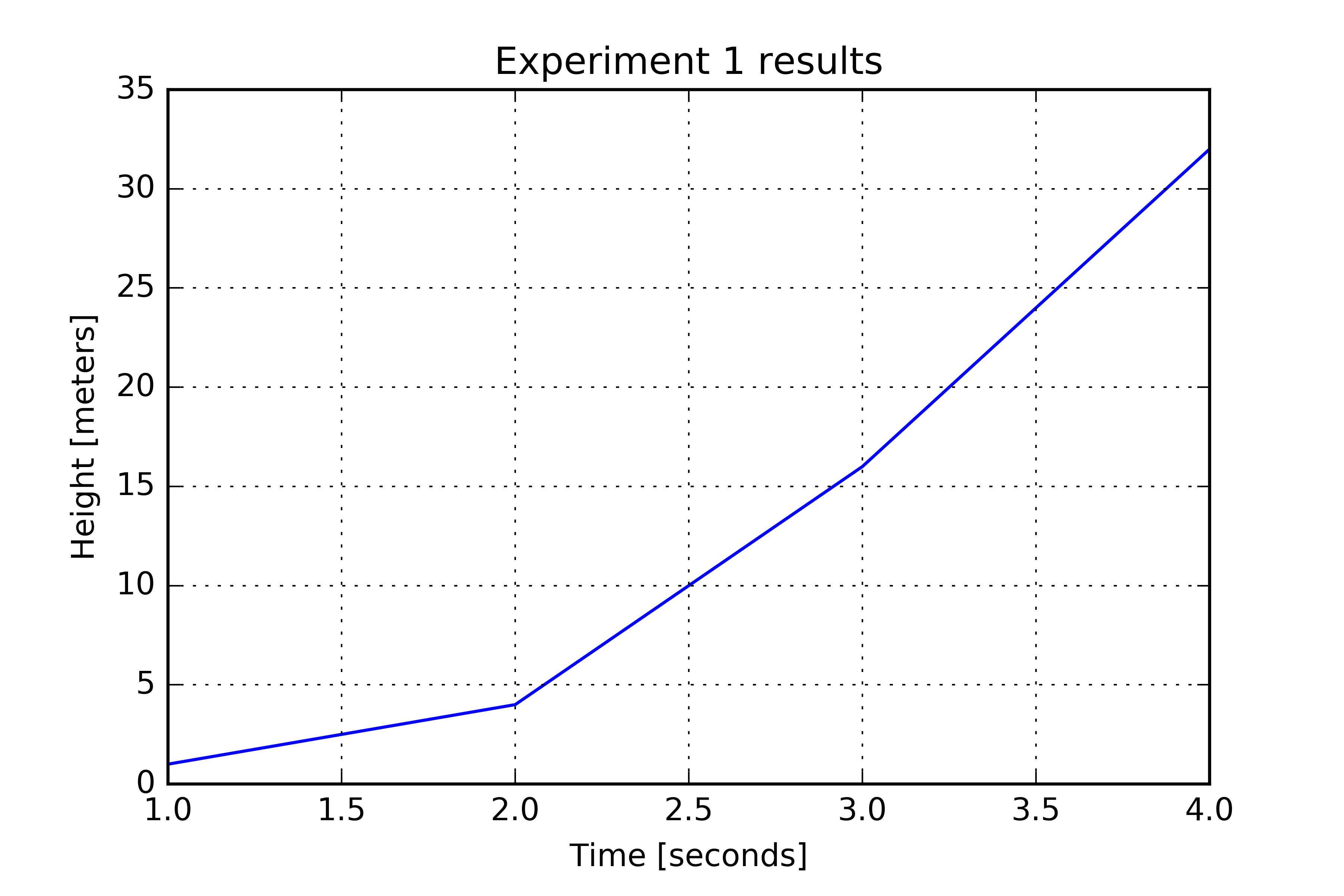

Matplotlib labels can be specified using TeX strings (this may code may not work, most likely due to a needed package not being installed – do a web search on the error message to figure out how to install the missing package). For example

# See above if this results in an error message.
import matplotlib.pylab as plt
y = [1, 4, 16, 32]
x = [1, 2, 3, 4]
plt.plot(x, y)
plt.grid()
plt.xlabel('Time [seconds]');
plt.ylabel('Height [meters]');
plt.title(r'$\mathbf{A}=3\hat{\mathbf{x}} + 4\hat{\mathbf{y}}; E=mc^2$')
plt.show()

See Matplotlib Gallery for additional information.

13.5 Line Color

A line color may be specified when calling the plot function. This set of commands will create a red line. Enter help(plt.plot) on the command line to see a table of all possible color abbreviations.

import matplotlib.pyplot as plt
y = [1, 4, 16, 32]
plt.plot(y, 'r')       # Red line; 'g' would produce green line
plt.plot(y, color='r') # Same result using alternative syntax
plt.show()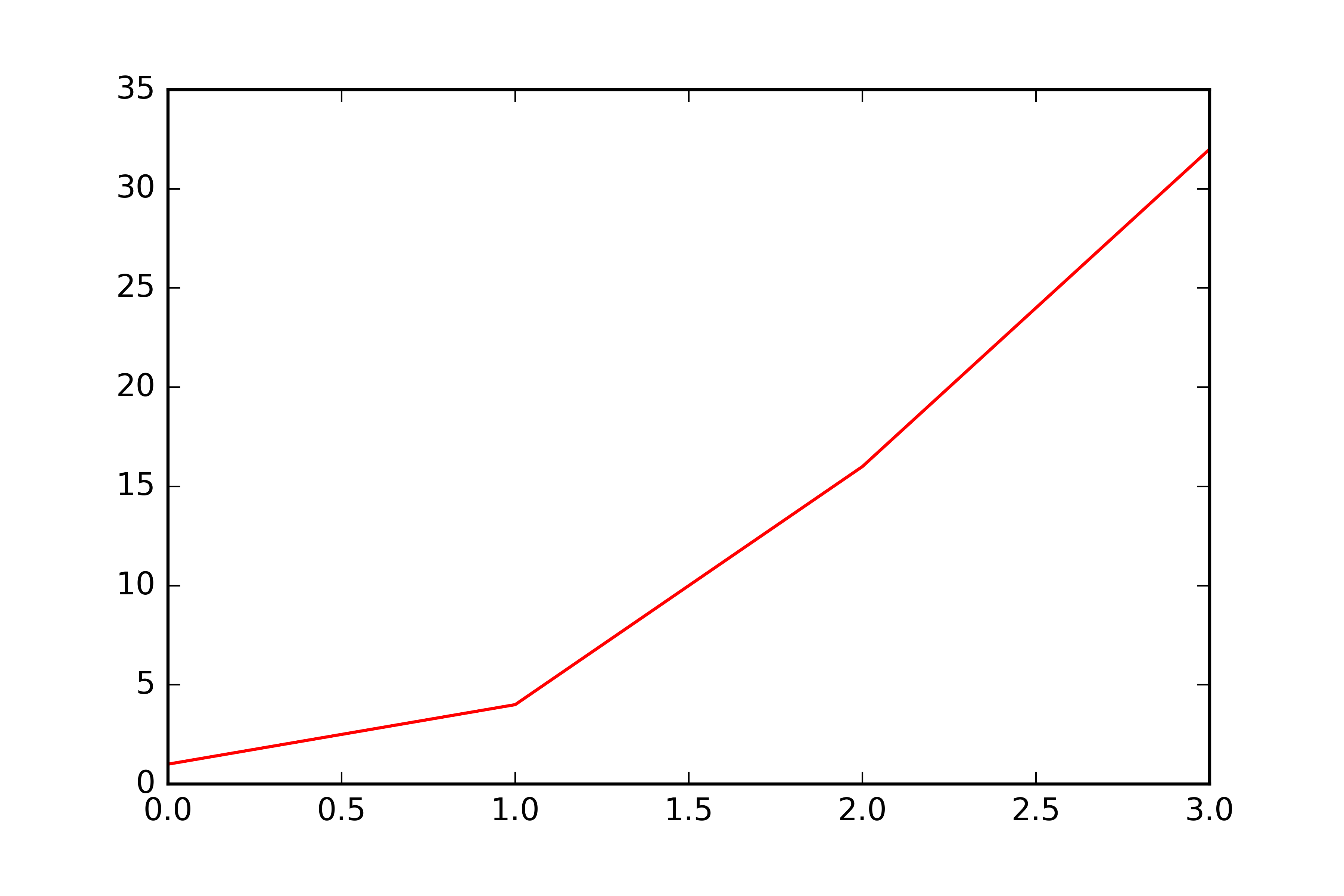

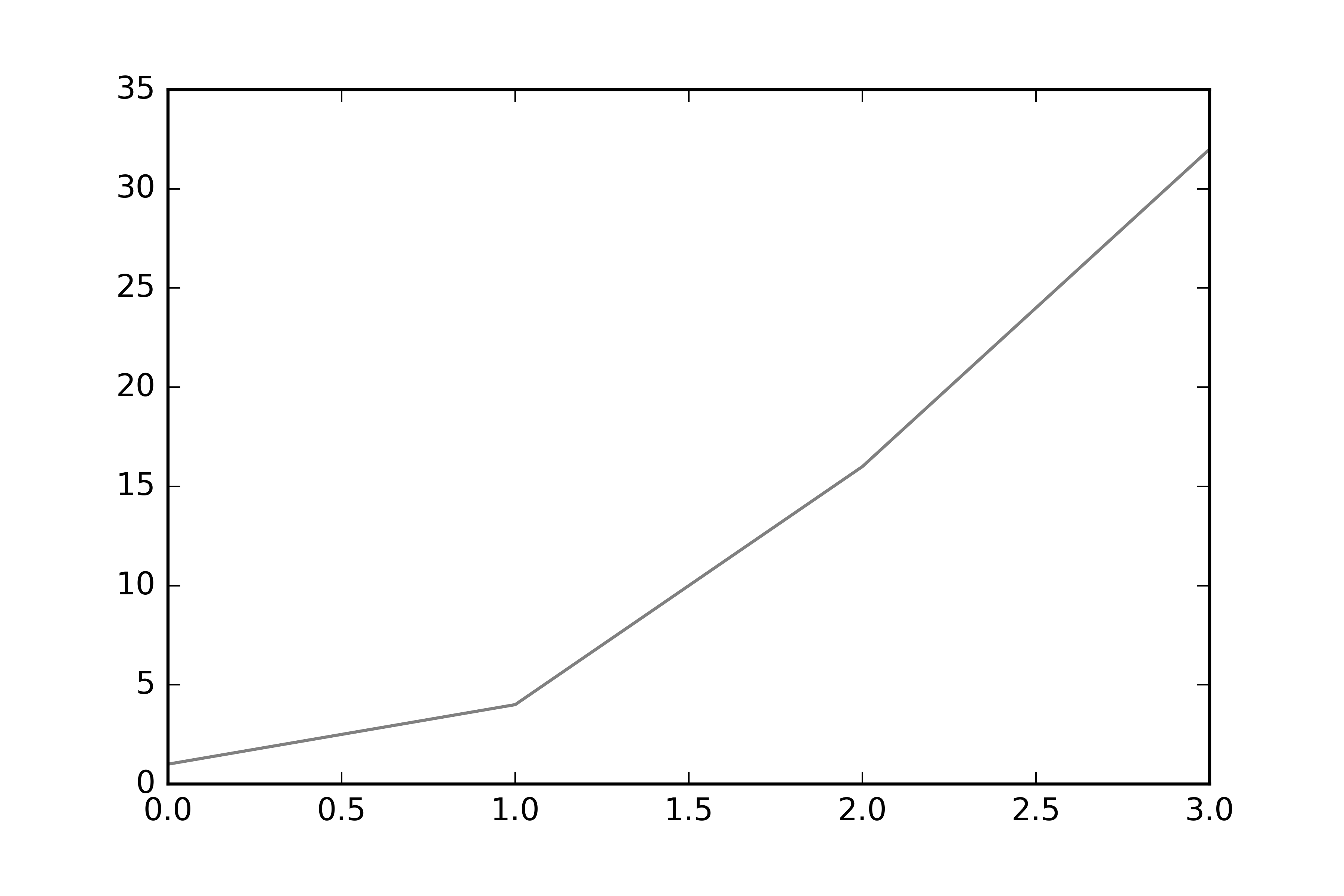
Colors that do not have an associated abbreviation may be used by specifying a list of red, green, and blue intensity values. This set of commands will create a gray line.

import matplotlib.pyplot as plt
y = [1, 4, 16, 32]
# 100% red intensity, 0% green, 0% blue
plt.plot(y, color=[1, 0, 0]) 
# Mixture of 50% red intensity, 50% green, and 50% blue
plt.plot(y, color=[0.5, 0.5, 0.5]) 
plt.show()

To find a special color, I usually do a search on, e.g., “rgb values for periwinkle”. Doing this, I find RGB: 204, 204, 255, which is translated to intensity fractions by dividing each number by 255, so I would use color=[204/255, 204/255, 255/255].

13.6 Line Style

By default, the points in y are connected with solid lines. Line styles options are solid, dashed, dashdot, dotted or their corresponding short-hand strings of -, :, -., -- can also be used.

import matplotlib.pyplot as plt
y = [1, 4, 16, 32]
plt.plot(y, '-', linewidth=5)
# or
plt.plot(y, linestyle='solid', linewidth=5)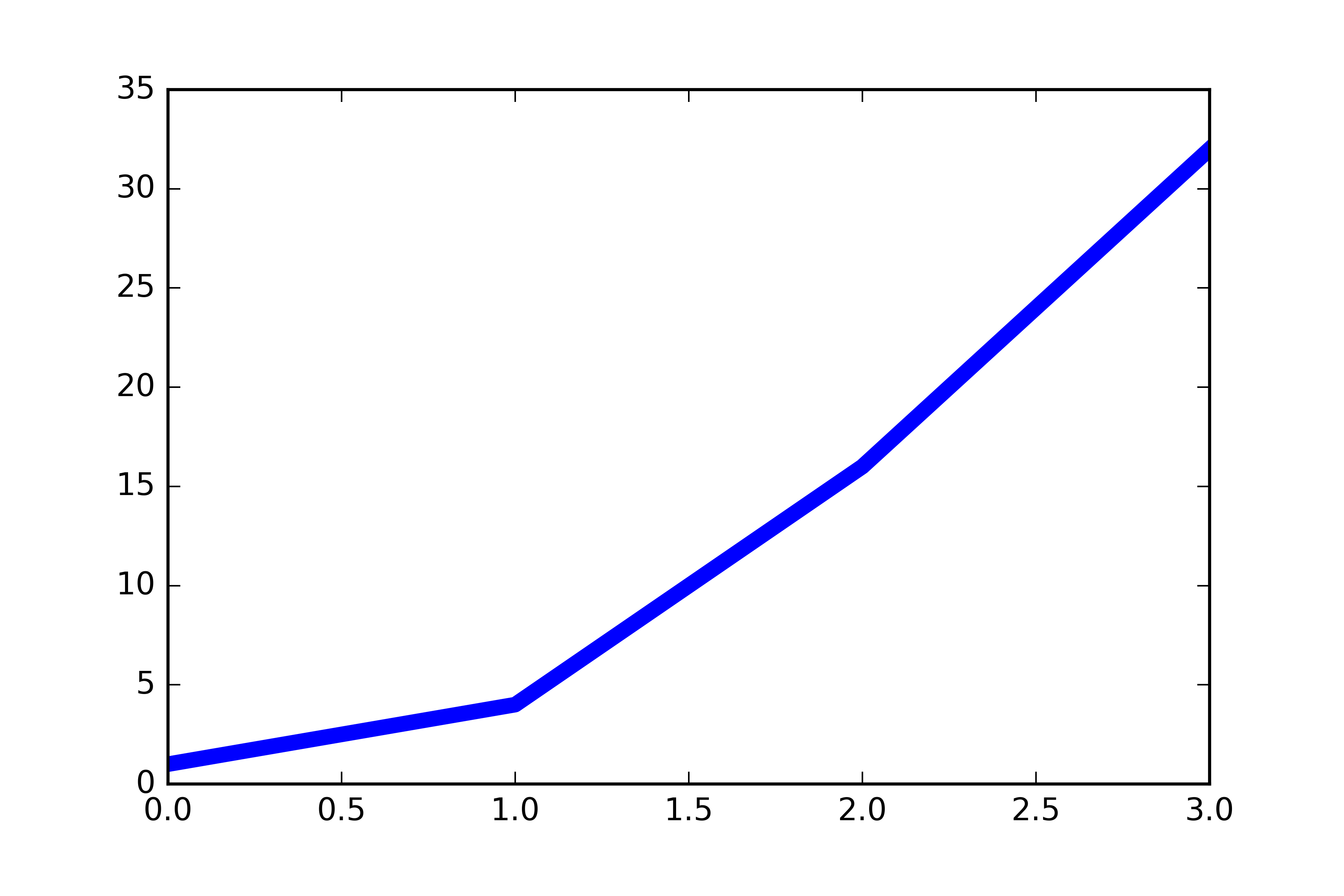

13.7 Marker Style

Instead of drawing connected lines, markers can be drawn at points. See help(plt.plot) for a table of possible markers.

import matplotlib.pyplot as plt
y = [1, 4, 16, 32];
plt.plot(y, '*') # Stars
#plt.plot(y, 'o') # Circles
plt.show()

url=https://raw.githubusercontent.com/rweigel/computingforscientists/master/Plotting_1D/figures/Plotting_1D_VII.py.png|width=400px|expire=1

Marker colors may be specified using the same syntax as the line color

import matplotlib.pyplot as plt
y = [1, 4, 16, 32]
plt.plot(y, '*', color=[0.5, 0.5, 0.5]) # Gray stars
plt.show()

url=https://raw.githubusercontent.com/rweigel/computingforscientists/master/Plotting_1D/figures/Plotting_1D_VIII.py.png|width=400px|expire=1

The marker size may be specified using markersize keyword

import matplotlib.pyplot as plt
y = [1, 4, 16, 32]
plt.plot(y, '*', markersize=10)
plt.show()

|style=”vertical-align:top”| url=https://raw.githubusercontent.com/rweigel/computingforscientists/master/Plotting_1D/figures/Plotting_1D_IX.py.png|width=400px|expire=1

13.8 Style Combinations

Multiple styles may be specified. For example, to create a red solid line, use r-

import matplotlib.pyplot as plt
y = [1, 4, 16, 32]
plt.plot(y, 'r-', linewidth=3)

url=https://raw.githubusercontent.com/rweigel/computingforscientists/master/Plotting_1D/figures/Plotting_1D_XII.py.png|width=400px|expire=1

To create a red solid line that connects points in y and to show stars at the points, use r*-

import matplotlib.pyplot as plt
y = [1, 4, 16, 32]
plt.plot(y, 'r*-', linewidth=3, markersize=10)
# or (a bit easier to read)
plt.plot(y, color='r', linestyle='solid', 
         marker='*', linewidth=3, markersize=10)

url=https://raw.githubusercontent.com/rweigel/computingforscientists/master/Plotting_1D/figures/Plotting_1D_XIII.py.png|width=400px|expire=1

13.9 Multiple lines and legends

To create a legend, use legend:

import matplotlib.pyplot as plt
A = [1.0, 4.0, 16.0, 32.0]
B = [1.1, 4.4, 16.9, 32.9]
l1, = plt.plot(A, 'b')
l2, = plt.plot(B, 'r')
plt.legend(['A', 'B'])
plt.show()

url=https://raw.githubusercontent.com/rweigel/computingforscientists/master/Plotting_1D/figures/Plotting_1D_XV.py.png|width=400px|expire=1

To set the legend location, use the loc keyword. See help(plt.legend) or [https://matplotlib.org/users/legend_guide.html] for other options:

import matplotlib.pyplot as plt
A = [1, 4, 16, 32]
B = [1.1, 4.4, 16.9, 32.9]
l1, = plt.plot(A, 'b')
l2, = plt.plot(B, 'r')
plt.legend(['A', 'B'], loc='upper left')
plt.show()

url=https://raw.githubusercontent.com/rweigel/computingforscientists/master/Plotting_1D/figures/Plotting_1D_XVI.py.png|width=400px|expire=1

13.10 Axis Tick Numbers

In the previous example, Matplotlib chose to label the values in 0.5 increments. This is not a good default for the plotted list - all of the x-values are integers. Use xticks and yticks to specify the tick labels to show.

import matplotlib.pyplot as plt
A = [1, 4, 16, 32]
plt.plot(A, 'r*-', linewidth=3, markersize=10)
plt.xticks([0,1,2,3])
plt.show()

To modify the y-position labels, use yticks instead of xticks.

url=https://raw.githubusercontent.com/rweigel/computingforscientists/master/Plotting_1D/figures/Plotting_1D_XVII.py.png|width=400px|expire=1

13.11 Axis Limits

In the previous examples, only part of the first and last markers were shown. To expand the axis limits so the full markers are shown, use plt.xlim()

import matplotlib.pyplot as plt
A = [1, 4, 16, 32]
plt.plot(A, 'r*-', linewidth=3, markersize=10)
plt.xticks([0, 1, 2, 3])
plt.xlim([-0.1, 3.1])
plt.show()

To modify the y-axis limits, use ylim.

url=https://raw.githubusercontent.com/rweigel/computingforscientists/master/Plotting_1D/figures/Plotting_1D_XVIII.py.png|width=400px|expire=1

13.12 `imshow`

The following program demonstrates how a matrix can be plotted.

#from matplotlib import cm
import numpy as np
# Create matrix to plot
z = np.array([[0, 1], [2, 3]])
print(z)
# Open a new figure
plt.figure()
# Create a colormap with 4 colors from white to black.
cmap = plt.get_cmap('Greys', 4)
# Plot the matrix z
im = plt.imshow(z, cmap=cmap)
# Set labels
plt.xlabel('column')
plt.ylabel('row')
# Set x- an y-ticks to be integers
plt.gca().set_xticks([0, 1])
plt.gca().set_yticks([0, 1])
# Show colorbar
cb = plt.colorbar()
# Set colorbar axis label
#cb.set_label('z') # Next to colorbar axis numbers
cb.ax.set_title('z') # Top of colorbar
# Set colorbar limits so colors are centered on integers
plt.clim(-0.5, 3.5)
# Set colorbar ticks
#cb.set_ticks([0, 1])
# dpi=300 (dots per inch) saves a higher resolution image than the default
# bbox_inches='tight' removes extra whitespace surrounding plot
plt.savefig('HW11_3_imshow.png', dpi=300, bbox_inches='tight')

14 datetimes

If you get an error related to “utc datetime.timezone”, remove tzinfo=timezone.utc. For example modify

t1 = datetime(1970, 1, 1, 
              hour=0, minute=0, second=0, 
              microsecond=0, tzinfo=timezone.utc)

to be

 t1 = datetime(1970, 1, 1, 
              hour=0, minute=0, second=0, 
              microsecond=0)

A datetime object is used to store dates and times. The datetime object methods allow a given datetime to be manipulated.

The advantage of using datetimes is

One can do math on them, e.g., find the number of days, hours, minutes, seconds between two dates.
A time that is stored as a datetime can be easily rendered in different ways, e.g., “2019-01-01” or “2019-001”.
When a list of datetimes is passed to Matplotlib’s plot function, it will automatically use date labels on the axes.

14.1 Basic Usage

In the following a datetime object t1 is created using the datetime function. The name of the module is datetime and one of the functions is datetime and the type of an object created by the function datetime is … datetime.

from datetime import datetime, timedelta, timezone
# Basic method for creating a datetime object
# Everything after the day (third argument) is optional
t1 = datetime(1970, 1, 1, 
              hour=0, minute=0, second=0, 
              microsecond=0, tzinfo=timezone.utc)
# Number of seconds since 1970-01-01 UTC
# (called the "POSIX Epoch")
print(t1.timestamp()) # 0.0
# Print timestamp in ISO 8601 format. 
# The +00:00 is the time zone offset.
print(t1.isoformat()) # 1970-01-01T00:00:00+00:00
t1 = datetime(1970, 1, 1, 
              hour=0, minute=30, second=0, 
              microsecond=0, tzinfo=timezone.utc)
# Number of seconds since 1970-01-01 UTC
print(t1.timestamp()) # 1800.0

I recommend always specifying the timezone as UTC unless you are dealing with local times. When all timezones are not UTC, you may run into surprises when the differences between two datetimess is computed. See [https://docs.python.org/3/library/datetime.html].

14.2 Creating Custom Time Strings

The format method used on strings has codes such as d, f, and e for representing a number as an integer, floating point number, or number in scientific notation. For example,

print("{0:f}".format(1.1)) # 1.100000

Similarly, the method strftime has specifiers for specifying how a date and time should be displayed. See [https://www.programiz.com/python-programming/datetime/strftime] for a full list of specifiers.

from datetime import datetime, timedelta, timezone
t1 = datetime(2019, 10, 23, 
              hour=1, minute=2, second=3, 
              microsecond=4, tzinfo=timezone.utc)
# Print timestamp using custom format
# See https://www.programiz.com/python-programming/datetime/strftime
# for list of codes
print(t1.strftime('%Y-%m-%d')) # 2019-10-23
print(t1.strftime('%m/%d/%Y')) # 10/23/2019
print(t1.strftime('%Y-%j'))    # 2019-296 (%j = day of year)
print(t1.strftime('%Y-%m-%d @ %H:%M:%S.%f')) # 2019-10-23 @ 01:02:03.000004

14.3 Time Deltas

A timedelta object represents the difference between two datetimes.

timedelta objects can be created using the timedelta function, e.g.,

from datetime import datetime, timedelta, timezone
# Create a timedelta object
dt = timedelta(days=1, seconds=0, microseconds=0)
# Print information
print(dt.days)            # 1
print(dt.seconds)         # 0
print(dt.microseconds)    # 0
print(dt.total_seconds()) # 86400.0

timedelta objects can be computed using two datetime objects, e.g.,

from datetime import datetime, timedelta, timezone
t1 = datetime(2019, 10, 23, 
            hour=0, minute=0, second=0, 
            microsecond=0, tzinfo=timezone.utc)
t2 = datetime(2020, 10, 23, 
            hour=0, minute=0, second=23, 
            microsecond=0, tzinfo=timezone.utc)
dt = t2 - t1
# Print information
print(dt.days)            # 366
print(dt.seconds)         # 23
print(dt.microseconds)    # 0
print(dt.total_seconds()) # 31622423.0

A timedelta can be added or subtracted from a datetime.

from datetime import datetime, timedelta, timezone
# Create a base datetime
t1 = datetime(2019, 10, 23, 
            hour=0, minute=0, second=0, 
            microsecond=0, tzinfo=timezone.utc)
print(t1.isoformat()) # 2019-10-23T00:00:00+00:00
dt = timedelta(days=1, seconds=44, microseconds=0)
# Add an increment to base datetime
t2 = t1 + dt
print(t2.isoformat()) # 2019-10-24T00:00:44+00:00

14.4 Creating a list of `datetimes`

Create a list with 10 datetime objects with a spacing of 1 day.

from datetime import datetime, timedelta, timezone
t1 = datetime(2019, 10, 23, 
            hour=0, minute=0, second=0, 
            microsecond=0, tzinfo=timezone.utc)
# Create a list with 10 datetime objects with a spacing of 1 day
dt = timedelta(days=1)
T = []
for i in range(10):
    t = t1 + i*dt
    T.append(t)
    # Display what was appended in string format
    ts = t.isoformat()
    print(ts)
print(T)
'''
2019-10-23T00:00:00+00:00
2019-10-24T00:00:00+00:00
2019-10-25T00:00:00+00:00
2019-10-26T00:00:00+00:00
2019-10-27T00:00:00+00:00
2019-10-28T00:00:00+00:00
2019-10-29T00:00:00+00:00
2019-10-30T00:00:00+00:00
2019-10-31T00:00:00+00:00
2019-11-01T00:00:00+00:00
[datetime.datetime(2019, 10, 23, 0, 0, tzinfo=datetime.timezone.utc),
 datetime.datetime(2019, 10, 24, 0, 0, tzinfo=datetime.timezone.utc),
 datetime.datetime(2019, 10, 25, 0, 0, tzinfo=datetime.timezone.utc),
 datetime.datetime(2019, 10, 26, 0, 0, tzinfo=datetime.timezone.utc),
 datetime.datetime(2019, 10, 27, 0, 0, tzinfo=datetime.timezone.utc),
 datetime.datetime(2019, 10, 28, 0, 0, tzinfo=datetime.timezone.utc),
 datetime.datetime(2019, 10, 29, 0, 0, tzinfo=datetime.timezone.utc),
 datetime.datetime(2019, 10, 30, 0, 0, tzinfo=datetime.timezone.utc),
 datetime.datetime(2019, 10, 31, 0, 0, tzinfo=datetime.timezone.utc),
 datetime.datetime(2019, 11, 1, 0, 0, tzinfo=datetime.timezone.utc)]
'''

In the previous example, we used range(10). A more likely use-case is that a start and stop datetime will be known, in which case the argument to range is better calculated from the difference between the start and stop datetimes.

from datetime import datetime, timedelta, timezone
to = datetime(2015, 1, 12, tzinfo=timezone.utc)
tf = datetime(2015, 2, 13, tzinfo=timezone.utc)
dt_span = tf - to
dt = timedelta(days=1)
T = []
for i in range(dt_span.days):
    t = to + i*dt
    T.append(t)
    # Display what was added in string format
    ts = t.isoformat()
    print(ts)
"""
2015-01-12T00:00:00
2015-01-13T00:00:00
2015-01-14T00:00:00
2015-01-15T00:00:00
...
2015-02-08T00:00:00
2015-02-09T00:00:00
2015-02-10T00:00:00
2015-02-11T00:00:00
2015-02-12T00:00:00
"""

14.5 Matplotlib and `datetimes`

Matplotlib will label any axis with datetime objects using a formatted string.

from datetime import datetime, timedelta, timezone
to = datetime(2015, 1, 12, tzinfo=timezone.utc)
dt = timedelta(days=1)
T = []
y = []
for i in range(10):
    t = to + i*dt
    T.append(t)
    y.append(i)
from matplotlib import pyplot as plt
plt.plot(T, y, '.')

Matplotlib is often not good at choosing how to label a time axis. Typically one needs to search for examples of how to modify them, e.g., [https://matplotlib.org/3.1.1/gallery/recipes/common_date_problems.html] or use a library that adds functionality to Matplotlib such as [Seaborn](https://matplotlib.org/3.1.1/gallery/recipes common_date_problems.html) or Bokeh.

14.6 Parsing Custom Time Strings

Quite often, one will have a list of time strings that need to be converted into a datetime object. The datetime module does not know how to do this unless the string is in the standard ISO 8601 format. However, most date and time strings you will encounter are not in this standard format. (The Pandas library has a function that can guess the format.)

from datetime import datetime
# Date given in Year-DOY (DOY = day of year, aka "Julian Day")
# This is a common format in astronomy-related data
t1 = datetime.strptime('1999-004', '%Y-%j')
print(t1.isoformat()) # 1999-01-04T00:00:00
# String in standard US format
t1 = datetime.strptime('10/31/2019', '%m/%d/%Y')
print(t1.isoformat()) # 2019-10-31T00:00:00
# Same date as above but in format used in other parts of the world
t1 = datetime.strptime('31/10/2019', '%m/%d/%Y')
print(t1.isoformat()) # 2019-10-31T00:00:00

Convert a list of date and time strings to a list of datetime objects.

from datetime import datetime
T_strings = ['1999-001', '1999-002', '1999-003']
T_objects = []
for ts in T_strings:
    t = datetime.strptime(ts, '%Y-%j')
    T_objects.append(t)
    print(t.isoformat())
"""
1999-01-01T00:00:00
1999-01-02T00:00:00
1999-01-03T00:00:00
"""

15 NumPy

15.1 Importing

At the start of any program that uses NumPy, import it using import numpy as np, e.g.,

import numpy as np
print(np.pi) # Prefix Numpy usage with np

As with Matplotlib’s import statement, the last string, in this case np, can vary

import numpy as npy # Sometimes npy used instead of np
print(npy.pi) # Prefix Numpy usage with npy

15.2 Arrays

The general-purpose data structure in NumPy is the ndarray (as in N-dimensional array). It is an analog to the Python list.

Whereas a list can contain values with different data types, a NumPy ndarray can only contain values with a single data type.

To review, a Python list can be created using the square bracket notation

L = [1, 2.1, 'zz'] # List with a mix of data types - int, float, and string
dir(L) # List all methods of L

The dir command lists all of the methods that apply to a list object such as append. (Ignore the ones that start with underscores for now.)

There are many ways to create a NumPy ndarray; the most basic uses the function array with an argument of a list.

import numpy as np
L = [1, 2, 3]
A = np.array(L) # Converts list L to a NumPy ndarray
type(A) # numpy.ndarray
dir(A) # List all methods of A

The list of methods and attributes displayed for the ndarray object A is much longer and contains mathematical operations such as dot, min, and max. Three of the key attributes that you will use are shape, size, and dtype:

import numpy as np
A = np.array([1, 2, 3])
print(A.shape) # (3, ) # Notation explained below
print(A.size)  # 3
print(A.dtype) # int64

A key restriction on a ndarray is that all elements are of the same data type. This is the reason that a ndarray can have a method max and min and why ndarrays can be multiplied and added. If a list contained strings and numbers, these operations are ill-defined.

import numpy as np
A = np.array([1, 2, 3])
print(L.max()) # Error b/c what is the max of 1, 2, and 'zz'?
# Error msg is "list object has no attribute 'max'".  
# This works as expected.
print(A.max()) # 3

15.3 Array Shape

The shape of a ndarray is the number of rows and columns and additional dimensions.

import numpy as np
M = np.array([[1, 2, 3], [3, 4, 5]]) # Create ndarray from list of lists
print(M)
print(M.shape) # (2, 3) - two rows, three columns

The shape of NumPy ndarray is a tuple, not a list. Because tuples cannot be modified, this serves as a hint that an operation such as s = M.shape; s[0] = 9 cannot be used to change the size of an array.

Going back to the first example, the trailing comma in the shape of (3, ) needs to be explained.

A = np.array([1, 2, 3])
print(A)
print(A.shape) # (3, )

Based on the matrix example, where M.shape = (2, 3), one may have expected A.shape to be (3) instead of (3, ). The short explanation is that the (3, ) can generally be interpreted as meaning the same as (3) and the trailing comma can be ignored.

Long answer

a tuple with one element such as (3) is the same thing as 3 in Python and
code that uses NumPy is simpler if A.shape is always a tuple.

To see point 1., consider

t = (3)
print(type(t)) # int
print(t[0]) # Error
len(t) # Error
t = (3, )
print(type(t)) # tuple
print(t[0]) # 3
len(t) # 1

As a compromise, the unintuitive notation (3, ) is used for the shape of 1-D NumPy arrays (and single-element tuples in general). The existence of the comma tells Python that the quantity in parenthesis is actually meant to be a tuple.

The reason that the Python interpreter can’t conclude (3) is a tuple is in math operations is it is acceptable to wrap a number in parenthesis and so I expect (3)*1 to mean 3*1 and not a tuple times a scalar.

15.4 Array Size

The size of an array is simply the number of elements. For example, a (3\times 2) array has (3\cdot 2) elements

import numpy as np
M = np.array([[1, 2, 3], [3, 4, 5]])
print(M.size) # 6

The size of an array could also be computed from the product of the elements in the shape tuple:

import numpy as np
M = np.array([[1, 2, 3], [3, 4, 5]])
N = M.size    # N = 6 
s = M.shape   # s = (3, 2)
N = s[0]*s[1] # N = 6
M = np.array([M, M]) # Create a 3-D array
N = M.size           # N = 12 
s = M.shape          # s = (3, 2, 2)
N = s[0]*s[1]*s[2]   # N = 12

15.5 Array dtype

Every NumPy array has a data type attribute dtype that indicates how the numbers are stored internally. When the np.array function is used to convert a list to a NumPy array, the chosen dtype depends on the elements in the list.

import numpy as np
A = np.array([1, 2, 3])
print(A.dtype) # int32
A = np.array([1., 2., 3.])
print(A.dtype) # float64

The data type can be explicitly set using the dtype keyword.

import numpy as np
A = np.array([1, 2, 3], dtype=np.float64)
print(A.dtype) # float64

There are many other possible dtypes – see the NumPy documentation. In general, using np.float64 is the safest choice.

15.6 Creating Arrays

15.7 Initializing Arrays

15.7.1 With NaNs

Arrays can be initialized with values other than zero and one. Probably the safest approach is to start with an ndarray of all NaN (Not-a-Number) values:

import numpy as np
A = np.full((3, ), np.nan) 
print(A)
# [nan nan nan]

The motivation for initialization with NaNs is that coding errors become more obvious. The following program intends to set a value to each element in an array and then print the sum, but there is an error so that the last value is never set. When executed, the sum nan is printed:

import numpy as np
A = np.full((4, ), np.nan)
for i in range(len(A)-1): # Error is that this should be len(A)
    A[i] = i
print(np.sum(A)) # nan - you know something went wrong

In contrast, if the values of A were initialized to zero, this coding error may not have been noticed:

import numpy as np
A = np.zeros((4, ))
for i in range(len(A)-1): # Error is that this should be len(A)
    A[i] = i
print(np.sum(A)) # 3, but should be 7

There are other initialization methods that should be considered if execution speed is a concern, e.g.,

import numpy as np
A = np.empty((3, )) # Multiply each element by NaN.
A[:] = numpy.nan # Set each element to NaN
# or
# A = np.full((3, ), np.nan)
# or
# A = np.empty((3, )) 
# A.fill(numpy.nan)

15.7.2 With Equally Spaced Values

The functions arange and linspace are both used to create an 1-D ndarray with equally spaced values.

Either of the two functions can be used to create arrays with equally spaced values, but the NumPy documentation recommends that

arange should only be used to create an ndarray with integer values, e.g., [1., 2., 3.]
linspace should be used to create an ndarray with non-integer values, e.g., [0.1, 0.2, 0.]

Important:

stop values are exclusive for arange (last value is stop-1)
stop values are inclusive for linspace (last value is stop)

arange

arange(stop) Gives [0, 1, ..., stop-1]
arange(start, stop) Gives [start, start+1, ..., stop-1]. stop > start is required to give non-empty result
arange(start, stop, step) When step is given, start and/or stop can be negative, as can step.

print(np.arange(5))        # [0 1 2 3 4]
print(np.arange(2, 5))     # [2 3 4]
print(np.arange(-2, 3))    # [-2 -1 0 1 2]
print(np.arange(-5, -1))   # [-5 -4 -3 -2]
print(np.arange(1, 6, 2))    # [1 3 5]
print(np.arange(6, 1, -2))   # [6 4 2]
print(np.arange(0, -10, -2)) # [6 4 2]
print(np.arange(-6, -9, -1)) # [-6 -7 -8]

linspace

linspace(start, stop) Gives 50 equally spaced values with a first value of start and last value of stop.
linspace(start, stop, num) Gives num equally spaced values with a first value of start and last value of stop.

print(np.linspace(0, 1, 5))  # [0. 0.25 0.5  0.75 1.]
print(0.25*np.arange(0, 5))  # [0. 0.25 0.5  0.75 1.]
print(np.linspace(0, 5, 5))  # [0. 1.25 2.5 3.75 5.]
print(np.linspace(0, 5, 6))  # [0. 1. 2. 3. 4. 5.]
print(np.linspace(0, -5, 6)) # [0. -1. -2. -3. -4. -5.]

Example

# Create B = [0, 0.1, 0.2, 0.3, 0.4, 0.5] using a for loop
B = np.zeros(6)
for i in range(len(B)):
    B[i] = i/10
print(B)
# Create B = [0, 0.1, 0.2, 0.3, 0.4, 0.5] using linspace and arange
B = 0.1*np.linspace(0, 5, 6)
# or
B = np.linspace(0, 0.5, 6)
# or
B = 0.1*np.arange(0, 6)

15.7.3 With Random Numbers

15.7.3.1 Gaussian (“Normal”)

randn and random.normal

To create a 100-element array with numbers drawn by selecting a random floating point value from a Gaussian (“normal”) distribution with a mean of 1.0 and standard deviation of 1.0, use randn:

A = np.random.randn(100)
print(np.mean(A)) # Should be close to 0.0
print(np.std(A)) # Should be close to 1.0

More generally, use np.random.normal(mean, std, size=N) to generate an array of size N with values drawn from a Gaussian with mean of mean and standard deviation of std.

mu = 100
std = 10
n = 200
np.random.normal(mu, std, size=n)

Multidimensional arrays can also be created

A = np.random.randn(3, 4)
print(A.shape) # (3, 4)

15.7.3.2 Uniform

rand and randint

To create a 100-element array with numbers drawn by selecting a random floating point in the half-open interval [0, 1.0), use rand:

A = np.random.rand(100)
print(np.mean(A)) # Should be close to 0.5

randint

To create a 100-element array with numbers drawn by randomly selecting an integer in a specified range, use randint.

A = np.random.randint(0, 101, (100, )) # Possible values are 0, 1, ..., 1000
print(np.mean(A)) # Should be close to 50.0

Multidimensional arrays can also be created

A = np.random.rand(3, 4)
print(A.shape) # (3, 4)
A = np.random.randint(0, 101, (3, 4))
print(A.shape) # (3, 4)

The way in which the shape of the array is specified for randint differs from rand and randn. The following all create a $M\times N\times L$ array with random numbers

M = 3
N = 4
L = 5
A = np.random.rand(M, N, L)
A = np.random.randn(M, N, L)
A = np.random.randint(0, 101, (M, N, L))

In the case of randint, the shape of the desired array is specified using a tuple.

15.8 Accessing Elements

TODO: Cover indexing vs. slicing.

import numpy as np
A = np.array([11,12,13])
x = A[[0,1]] # x is new array
y = A[0:2]   # y is reference to elements 0 and 1 of x
x[0] = 99
print(A)    # [11 12 13]
y[0] = 99
print(A)    # [99 12 13]

1-D

For 1-D NumPy ndarrays, the syntax is similar to that for lists

import numpy as np
A = [11,12,13]
x = np.array(A)
print(A[0])
# 11
print(x[0])
# 11
print(A[0:2])
# [11, 12]
print(x[0:2])
# [11 12]

2-D

For 2-D and higher dimensions, NumPy uses a different syntax than that used for Python lists. To access element i, j of a NumPy ndarray A, use A[i, j]. This syntax will not work for a 2-D list.

import numpy as np
# Create a 2-D NumPy ndarray
x = np.array([[11,12,13],[14,15,16]])
print(x)
#[[11 12 13]
# [14 15 16]]
print(x.shape) # (2, 3)
print(x[0,0]) # row 0, col 0
# 11
print(x[0,1]) # row 0, col 1
# 12
x[0,1] = 99
print(x)
#[[11 99 13]
# [14 15 16]]

A common programming pattern is to iterate over each element in a matrix and print out its value.

import numpy as np
x = np.array([[11,12,13],[14,15,16]])
print(x)
#[[11 12 13]
# [14 15 16]]
print('i j x[i,j]') # print header
# x.shape = (2, 3), so
# x.shape[0] = 2
# x.shape[1] = 3
for i in range(x.shape[0]): # iterate over rows
    for j in range(x.shape[1]): # iterate over columns
        print("{0:d} {1:d} {2:d}".format(i, j, x[i,j]))
print(x)
# i j x[i,j]
# 0 0 11
# 0 1 99
# 0 2 13
# 1 0 14
# 1 1 15
# 1 2 16

15.9 Modifying Elements

1-D

15.9.1.1 With Loop

The syntax for modifying a 1-D NumPy ndarrays is similar to that was used for lists:

import numpy as np
t = np.zeros(5)
for i in range(5):
    t[i] = i
print(t) # [0. 1. 2. 3. 4.]

The above can be compared with the method that would be used to create and modify t using lists.

# Create a list
t = []
for i in range(5):
    t.append(0)
print(t)
# [0, 0, 0, 0, 0]
# Modify an existing list
for i in range(5):
    t[i] = i
print(t)
# [0, 1, 2, 3, 4]

15.9.1.2 Without Loop

import numpy as np
a = np.array([1,2,3,4,5,6,7,8,9,10], dtype=np.float)
a[0:3] = 99 # Set value of elements 0, 1, 2 to 99
print(a)    # [99. 99. 99.  4.  5.  6.  7.  8.  9. 10.]
a[ a >= 99 ] = np.nan # Replace 99s with np.nan
print(a)    # [nan nan nan  4.  5.  6.  7.  8.  9. 10.]
print(np.nansum(a))

2-D

import numpy as np
A = np.array([[1,2,3],[4,5,6]], dtype=np.float)
print(A.size)   # 6
print(A.shape)  # (2, 3)
A[0,1:3] = 99   # Set values in row 0, columns 1 and 2 to 99
print(A)
# [[ 1. 99. 99.]
# [ 4.  5.  6.]]

15.10 Finding Elements

An example of finding elements is

import numpy as np
A = np.array([1,2,3,4,5])
idx = A < 3
print(idx)      # [True True False False False]
B = A[idx]
print(B)        # [1 2]

If only the number of elements in A that match the constraint is desired, any of the following can be used

N = np.sum(idx)             # True is treated as 1, False as 0
N = len(idx[idx == True])
N = len(B)

The above is equivalent to the following

import numpy as np
A = np.array([1,2,3,4,5])
idx = np.empty(np.shape(A), dtype=np.bool)
B = []
for i in range(A.size):
    if A[i] < 3:
        B.append(A[i])
        idx[i] = True
    else:
        idx[i] = False
B = np.array(B)
print(idx)      # [True True False False False]
print(B)        # [1 2]
print(len(B))   # 2

Alternatively, np.where can be used. The syntax is

np.where( condition, value if condition true, value if condition false)

The problem solved earlier using np.where is

import numpy as np
A = np.array([1, 2, 3, 4, 5])
B = np.where( A < 3, 1, 0)
# In locations where A  < 3, B will have the value of 1
# In locations where A >= 3, B will have the value of 0
print(B)        # [1,1,0,0,0]
print(sum(B))   # 2

Compound conditions can be evaluated using np.logical_and(). For example, to find elements in A in the range [2,4]

import numpy as np
A = np.array([1, 2, 3, 4, 5])
B = np.where(np.logical_and( A >= 2, A <= 4), 1, 0)
print(B) # [0 1 1 1 0]

To return the indices, use np.nonzero(), e.g.,

import numpy as np
A = np.array([1, 2, 3, 4, 5])
B = np.asarray( A > 2).nonzero()[0]
print(B) # array([2, 3, 4])

16 Statistics

16.1 Histograms

The syntax for the histogram function in Matplotlib is demonstrated in this example.

import matplotlib.pyplot as plt
import numpy as np
mu = 80.
sigma = 7.
n = 2000
x = np.random.normal(mu, sigma, size=n)
# Default; Should almost never use. Default bin choices are usually poor.
plt.hist(x)
# Expected peak is at 80. Create bins with edges at 45, 47, ..., 113
# so that centers are at 46, 48, ..., 80, ..., 112
plt.figure()
bins = np.arange(45,115,2)
print(bins)
plt.grid(axis='y')
plt.hist(x, bins=bins)
plt.title('$\mu= %.2f$, $n=%d$, $\overline{X} = $ %.2f' % (mu, n, np.mean(x)))
plt.xlabel('$X$')
plt.ylabel('# in bin')