1 HW 1

Due September 5th at 11:59 pm.

If you are stuck, please ask questions on Discord or send me questions via email.

Turn in all of your answers on paper.

1.1 Continuous Charge Distribution Approximation

In E&M, we often assume that point charges are continuously distributed. This problem addresses the accuracy of this approximation.

A line of length $2L$ is centered on the origin and lies between $-L\le x\le L$. The charge density, ${\lambda }_o$, on the line is uniform.

If the line is approximated by an odd number of point charges (so a charge is always at the origin) separated by a distance $\Delta$ and is used to compute the approximate electric field $E_{ya}$ on the $y$-axis at $y=L$, how many charges are required so that

$$\left|\frac{E_{ye}(0,L)-E_{ya}(0,L)}{E_{ye}(0,L)}\right|\le 0.01$$

where the exact solution is given by $E_{ye}$.

You may look up the exact solution but cite your source. You may use any program or a calculator to solve this problem.

Print out the code you used for your answer and write the actual answer it yields in a comment.

Save your program as a file named HW1_1.ext, where ext is the file extension for your program, e.g., m, py, etc. You do not need to send me your code (unless you have a question about it), but in the future, I’ll have you use GitHub to store your code with that filename.

Solution

Assume a charge at x of $\lambda dx$, with $dx$ small enough to be such that it is effectively a point charge. If this is the case, the vector from $x$ to $y=h$ is $\mathbf{r}=-x\hat{\mathbf{x}}+y\hat{\mathbf{y}}$ and so

$$d\mathbf{E}=k(\lambda dx)\hat{\mathbf{r}}/r^2=k(\lambda dx)\mathbf{r}/r^3=k(\lambda dx)(-x\hat{\mathbf{x}}+y\hat{\mathbf{y}})/r^3$$

To find the electric field due to a summation of these charges at $x$ from $-L$ to $L$, integrate the above expression.The exact solution is (Griffiths 4th Edition, example 2.2):

$$E_y=2k{\lambda }_{o}L\frac{1}{y\sqrt{y^2+L^2}}$$

We want to re-write this is a form that will allow cancellation of constants that were not given when the above ratio is computed. Using ${\lambda }_o=Q/2L$, we have

$$E_y=\frac{kQ}{L^2}\frac{1}{\frac{y}{L}{\left[1+{\left(\frac{y}{L}\right)}^2\right]}^{1/2}}$$

With $y=L$,

$$E_y=\frac{kQ}{L^2}\frac{1}{\sqrt{2}}$$

For a charge $Q$ at position $(x,y)$

$$E_y=kQ\frac{y}{(y^2+x^2{)}^{3/2}}$$

Setting $y=L$, this can be written as

$$E_y=\frac{kQ}{L^2}\frac{1}{{\left[1+{\left(\frac{y}{L}\right)}^2\right]}^{3/2}}$$

To compute the field due to multiple charges, we need to place charges at $x=-L,-L+\Delta ,\dots ,L$. The spacing $\Delta /L$ is $2/(N-1)$.

With $kQ/L^2$ term omitted, the sum is

$$S(N)\equiv \frac{1}{N}\sum _{i=-(N-1)/2}^{(N-1)/2}\frac{1}{{\left[1+(i\Delta {)}^2\right]}^{3/2}}$$

Before implementing, check that this sum is correct by expanding it for $N=3$, $N=5$.

Important: I want to see checks like this in your code. In analytical problems you should always use limits to check answer. In numerical problems, you should always use some sort of check on a reduced problem to check your implementation. The following checks took me some time, but because I had them, I was able to catch errors very quickly and also have confidence in my result. In my code, I also created two plots to help me build confidence in my result; see below. I plotted the sum as a function of $N$ and verified that it converged to a constant value (initially it did not, because I forgot to divide sum by $N$). I also plotted the error as a function of $N$ to verify that it was monotonically decreasing. (If it started increasing at some value of $N$, I would know that something went wrong.)

$N=3$, $\Delta =1$ and we want the sum terms to correspond to charges at $x/L=-1,0,$ and $1$.

$$S(N)=\frac{1}{3}\sum _{i=-1}^1\frac{1}{{\left[1+(i\Delta {)}^2\right]}^{3/2}}=\frac{1/3}{{\left[1+(-1{)}^2\right]}^{3/2}}+\frac{1/3}{{\left[1+(0{)}^2\right]}^{3/2}}+\frac{1/3}{{\left[1+(1{)}^2\right]}^{3/2}}$$

The result is $0.569035593728849$. This value is used in the following program as a check.

$N=5$, $\Delta =2/(N-1)=1/2$ and we want charges at $x/L=-1,-1/2,0,1/2,$ and $1$.

$$S(N)=\frac{1}{5}\sum _{i=-2}^2\frac{1}{{\left[1+(i\Delta {)}^2\right]}^{3/2}}=\frac{1/5}{{\left[1+(-1{)}^2\right]}^{3/2}}+\frac{1/5}{{\left[1+(-1/2{)}^2\right]}^{3/2}}+\frac{1/5}{{\left[1+(0/2{)}^2\right]}^{3/2}}+\frac{1/5}{{\left[1+(1/2{)}^2\right]}^{3/2}}+\frac{1/5}{{\left[1+(1\Delta {)}^2\right]}^{3/2}}$$

The result is $0.627638057357283$.

Notice the fact that the first two and last two terms evaluate to the same value. This can be used to reduce the number of computations.

To finish the problem, evaluate

$$\left|\frac{1/\sqrt{2}-S(N)}{1/\sqrt{2}}\right|\le 0.01$$

or $|1-\sqrt{2}S(N)|\le 0.01$

for odd positive values of $N$ until the inequality is satisified. The result should be $N=51$.

The following two figures were used to check my algorithm. Source code

1.2 Charge on Cylinder

Charge is uniformly distributed on the curved surface of a cylinder of length $h$ and radius $R$. The cylinder is centered on the origin, aligned with the $z$–axis, and has a uniform charge density of ${\sigma }_o$.

Find $\mathbf{E}(z)$. Prior to doing any calculations, document limiting cases that you can use to check your answer.

Answer

Limiting cases:

• Expect zero at origin.

  115

• Expect ring of charge solution as $h/R\to 0$

  116

• Expect infinite cylinder solution when $h\gg R$

  117

We also expect $E_z(z)=-E_z(z)$ (symmetry)

The field for uniformly charged ring in the $x$–$y$ plane and centered on the origin is

$$E_z=2\pi R\lambda k\frac{z}{{\left(z^2+R^2\right)}^{3/2}}=kQ\frac{z}{R^3}\frac{1}{{\left(1+(z/R{)}^2\right)}^{3/2}}$$

If the ring is translated along the $z$–axis by $z^{\prime }$, this corresponds to a translation of the coordinate system and we can write

$$E_z=\frac{kQ}{R^2}\frac{\left(\frac{z-z^{\prime }}{R}\right)}{{\left(1+{\left(\frac{z-z^{\prime }}{R}\right)}^2\right)}^{3/2}}$$

If we consider differential rings of height $d{z}^{\prime }$, their area is $2\pi Rd{z}^{\prime }$ and charge is

$dQ=(2\pi Rd{z}^{\prime }){\sigma }_o$

Replacing $E_z$ with $d{E}_z$ and $Q$ with $dQ$ in the last equation for $E_z$, we have

$$d{E}_z(z)=2\pi Rk\frac{d{z}^{\prime }}{R^2}\frac{\left(\frac{z-z^{\prime }}{R}\right)}{{\left(1+{\left(\frac{z-z^{\prime }}{R}\right)}^2\right)}^{3/2}}$$

and this must be integrated from $z^{\prime }=-h/2$ to $z^{\prime }=h/2$. The result is

$$E_z(z)=\frac{kQ}{R^2}\left[\frac{1}{h_R\sqrt{(\frac{z}{R}-\frac{h_R}{2}{)}^2+1}}-\frac{1}{h_R\sqrt{(\frac{z}{R}+\frac{h_R}{2}{)}^2+1}}\right]$$

where $h_R\equiv h/R$.

(The solution was written in this form in anticipation for a problem on HW #2.)

Checks:

• $E_z(0)=0$ is satisfied.

  153

• We expect ring of charge solution as $h/R=h_R\to 0$. However, when we plug this into the above, we get $1/0-1/0$, which is indeterminate.

  154

• Expect infinitely long and uniformly charged cylinder solution when $h\gg R$ (or $h_R\gg 1$). When we plug this into the above, we get $0$. This can be shown to be correct using Gauss’s law, from which it follows that $E_z=0$ at all points inside the cylinder (not only along $z$–axis, which we computed above).

  155

The symmetry condition $E_z(z)=-E_z(z)$ is satisifed.

Addressing the last two limits requires a significant amount of effort (see related problem). In the next homework, you will consider an alternative approach.

1.3 Reading

Next week, Gauss’s law will be covered. Find at least one freshman–level textbook and read the sections that cover Gauss’s law. Do the same for at least one upper–division undergraduate–level textbook (the references on the syllabus has a list of textbooks, but you may pick your own).

In the next class,

• We will have a general discussion on the similarities and differences in how Gauss’s law is presented and explained.

  167

• I will randomly select students (or groups) to present the solution to a problem of your choosing on the whiteboard. Prepare notes for a 5–7 minute presentation (no PowerPoint, only hand–written notes). During your presentation, I will ask the class for clarifications and connections to other problems. You are welcome and encouraged to work with one or two other students on this. Stated a different way, I would like you to review Gauss’s law from multiple sources, pick a problem you think you can explain (it can be a textbook example problem, in which case explain it in your own words), and prepare a short presentation of the solution. We’ll find that all solutions (even textbook examples) have many subtleties.

  168

Turn in your notes that you have prepared for a presentation.

2 HW 2

Due September 12th at 11:59 pm. Due to the fact that I forgot to post this on time, if you need an extensison, feel free to ask.

Upload your solutions to GitHub. Name all files associated with your solution as HW2_x.EXT, where x = 1, 2, 3, 4 is the problem from this homework and EXT is the file extension, e.g., pdf, py, m. Upload all files associated with your solution such as code and notes (in PDF).

If you are stuck, please ask questions on Discord or send me questions via email. Be prepared to answer questions about your answers to these problems. Even if you have not completed them, I will ask for your ideas on how to approach them.

2.1 Limiting Behavior For Cylinder

In the previous HW, you computed the electric field along the centerline of a cylinder with a uniform surface charge on its curved surface.

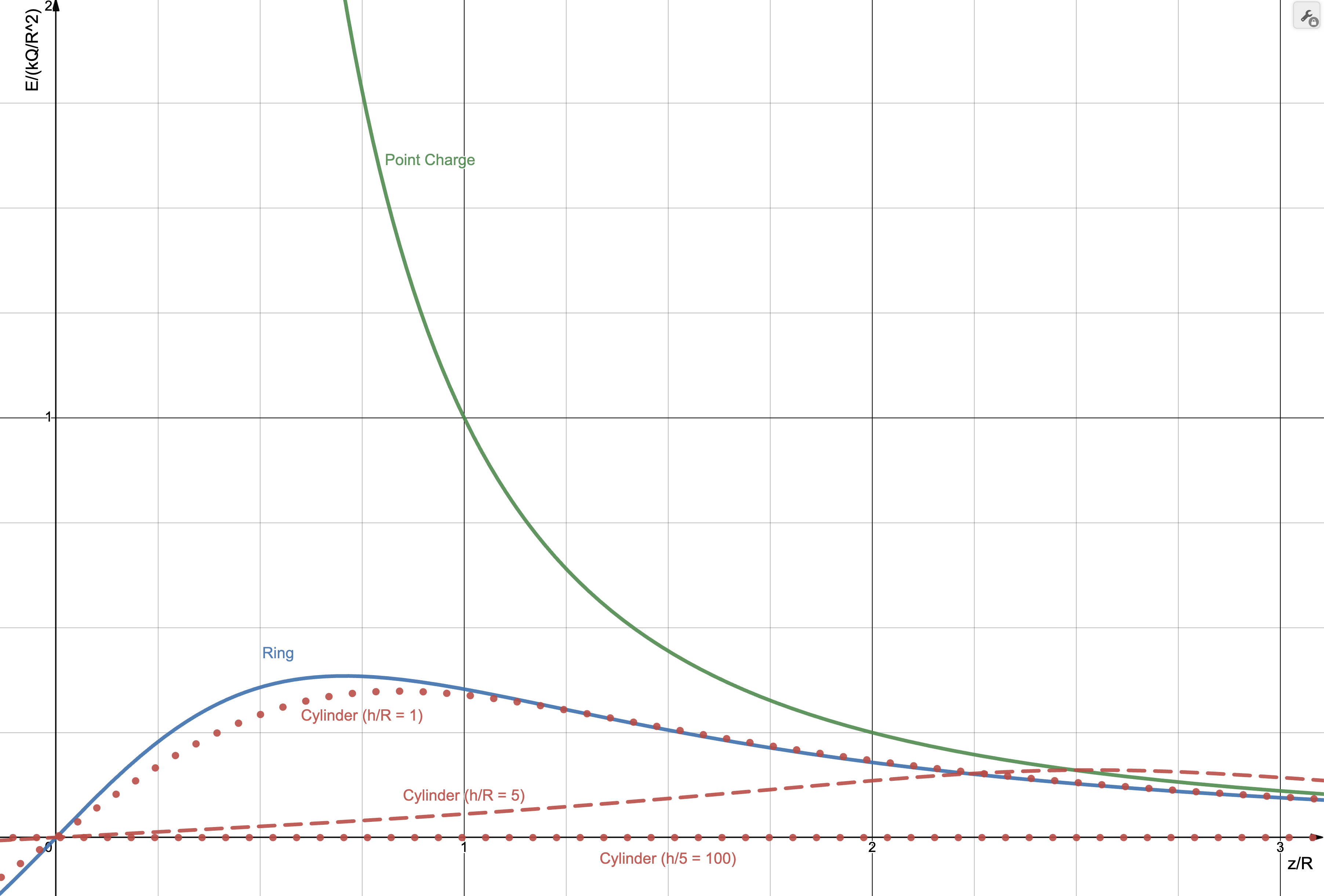
Showing that the equation approaches the equation for a point charge at the origin when $z\gg R$ and $z\gg h$ is not trivial. (Plugging $R=0$ and $h=0$ gives $E_z(z)=0$.) To show that $E_z(z)$ has the correct limiting behavior mathematically is quite involved. As an alternative, we will check the limit graphically.

Create a plot of $E_z(z/R)/E_o$, where $E_o=kQ/R^2$ for (that is, plot $E_z/E_o$ vs $z/R$):

1. A point charge $Q$ at the origin

   189

2. A ring of radius $R$ that is centered on the origin and lies in the $x$–$y$ plane with a uniformly distributed charge $Q$.

   190

3. The cylinder considered on the previous homework assuming for three cases: $h/R=1$, $h/R=5$, and $h/R=100$.

   191

Be prepared to provide a physical explanation for the features of the curves and the ratios of $h/R$.

• By using the dimensionless ratio, we can easily compare the fundamental features of the cylinder equation using only one parameter. If instead we plotted $E$ vs $z$, we would need to plot the equation for many values of $R$ and $h$ to understand the full range shapes the equation can have.\htmlnewline

  202

• As $h/R$ decreases, the cylinder solution approaches the ring solution. For $h/R=0.1$, the lines for the ring and cylinder cannot be distinguished by eye.\htmlnewline

  203

• For $h/R=1$, the cylinder and ring curves increasingly overlap starting at approximately $z/R=1$. This means the cylinder field is becoming more and more like the ring field as $z/R$ increases, which is expected.\htmlnewline

  204

• The ring and cylinder curves (for $h/R=1$) overlap with the point charge curve for large $z/R$. This is expected because both being to “look” like a point charge as you move away from them.\htmlnewline

  205

• The explanation for the curve approaching zero as $r/R$ increases is in this limit, the cylinder appears to be “long”. Inside of an infinitely long cylinder $h/R\to \infty$, the field is zero (even off–axis). This can be shown by using Gauss’s law.\htmlnewline

  206

• All curves have odd symmetry ($E(-z)=-E(z)$), as expected – the field for $z>0$ is positive and the field for $z<0$ is negative. (The image below only shows $z/R>0$.)\htmlnewline \htmlnewline \htmlnewline %

  207-210

2.2 Checking Gauss’s Law

Given a point charge $Q$ at the origin, compute the electric flux ${\Phi }_E=\int \mathbf{E}\cdot d\mathbf{A}$ through one face of a cube that is also centered on the origin using Coulomb’s law and explicit evaluation of the integral.

2.3 Charge on Concentric Thick Shells

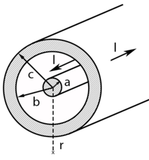
Charge placed on concentric spherical conducting shells, the cross–section of which is shown. Both shells have a thickness of $t$. The inner shell has an outer radius of $a$ and a net charge of $-Q$. The outer shell has an inner radius of $b$ and a net charge of $+Q$. Assume that $Q$ is positive.

Using Gauss’s law and the fact that the electric field inside a conductor must be zero show that

1. there can be no charge on the inner surface of the inner conductor,

   257-258

   Answer: A Gaussian sphere with a surface inside the inner conductor has $E=0$ on its surface (b/c $E$ inside a conductor is zero). Based on $\oint \vec{\mathbf{E}}\cdot d\mathbf{l}=Q_{\text{encl}}/{ϵ}_o$, this implies $Q_{\text{encl}}=0$. (Note that all charges must be on the surface of a conductor, so the only possible location for the charge is on the inner and outer surfaces.)

   259

2. the charge on the inner surface of the outer conductor is $+Q$, and

   261-262

   Answer: A Gaussian sphere with its surface inside the outer conductor has $E=0$ on its surface (b/c $E$ inside a conductor is zero). Based on $\oint \vec{\mathbf{E}}\cdot d\mathbf{A}=Q_{\text{encl}}/{ϵ}_o$, this implies $Q_{\text{encl}}=0$. The charge on the inner conductor was given as $-Q$. To make the charge inside the Gaussian sphere zero, we need $+Q$ on the inner surface of the outer conductor to get $Q_{\text{encl}}=0$.

   263

3. there is no charge on the outer surface of the outer conductor.

   265-266

   Answer: If the total charge on the outer conductor is $+Q$ and all of it is on its inner surface, but conservation of charge, there is no charge on its outer surface. Recall that charges arrange themselves on a conductor to make the electric field inside all conductors zero. With this charge arrangement, the field due to the charges on the outer surface of the inner conductor cancels the field due to the charge on the inner surface of the outer conductor for $r>b$.

   267

4. Find the electric field in each of the five labeled regions and sketch a plot of $E/(kQ/a^2)$ versus $r/a$. Region 1. is the empty volume inside of the inner conductor, region 2. is the inner conductor, region 3. is the empty volume between the conductors, region 4. is the outer conductor, and region 5. is the region outside of the outer conductor. (Hint: Use Gauss’s law several times; when not zero, the electric field should be proportional to $1/r^2$.)

   269-270

   Answer: 1. $E=0$ 2. $E=0$ 3. $E/(kQ/a^2)=-1/(r/a{)}^2$ 4. $E=0$ 5. $E=0$

   271

2.4 Scalar Potential

Because the electric field has the form of $\hat{\mathbf{r}}/r^2$, it can be shown that we can always find a scalar function $\psi$ (which we call electric potential) such that

$$\mathbf{E}=-\nabla \psi =-\frac{\partial \psi }{\partial x}\hat{\mathbf{x}}-\frac{\partial \psi }{\partial y}\hat{\mathbf{y}}-\frac{\partial \psi }{\partial z}\hat{\mathbf{z}}$$

It can be shown that this equation can be inverted:

$$\psi (\mathbf{r})-\psi ({\mathbf{r}}_o)=-{\int }_{{\mathbf{r}}_o}^{\mathbf{r}}\mathbf{E}\cdot d\mathbf{l}$$

where the integral is taken over any path between the points given by $\mathbf{r}$ and ${\mathbf{r}}_o$.

In one dimension, assuming the integration path is radial, and choosing ${\mathbf{r}}_o$ to be the origin, we have

$$\psi (r)-\psi (0)=-{\int }_0^r{E}_r(r)dr$$

Using the electric field from problem 2.3.4 and assuming $\psi (0)=0$ (I will discuss why this choice is arbitrary in class), find and sketch a plot of $\psi /(kQ/a)$ versus $r/a$.

In class, I will ask for a physical explanation for why I will get the same result if I choose a different integration path. For example, if my integration path was radial, then tangential, then radial again. This is covered in most intro textbooks. I’ll also ask why I ask for plots of dimensionless parameters in this problem and in other problems on this HW.

Solution

In region 1, $\psi (r)-\psi (0)=-{\int }_0^{r}0dr\Rightarrow \psi (r)=0$ and $\psi (a-t)=0$.

In region 2, $\psi (r)-\psi (a-t)=-{\int }_{a-t}^{r}0dr\Rightarrow \psi (r)=0$ and $\psi (a)=0$.

The fact that the potential is constant in region 2. is consistent with the expectation that a conductor is an equipotential.

In region 3, $\psi (r)-\psi (a)=kQ{\int }_a^{r}1/r^{\prime 2}d{r}^{\prime }\Rightarrow \psi (r)=kQ(1/a-1/r)$ and so $\psi (b)=kq(1/a-1/b)$

In region 4., the potential will be the same as in region 3. because a conductor is an equipotential: $\psi (r)=\psi (b)$

In region 5., assuming the outer radius of the outer shell is $c$, $\psi (r)-\psi (c)=-{\int }_c^{r}0dr\Rightarrow \psi (r)=\psi (c)$. Because $\psi (r)$ in region 4. is constant and equal to $\psi (b)$, $\psi (c)=\psi (b)$.

3 HW 3

Due September 19th at 11:59 pm.

Upload your solutions to GitHub. Name all files associated with your solution as HW3_x.EXT, where x = 1, 2, 3 is the problem from this homework and EXT is the file extension, e.g., pdf, py, m. Upload all files associated with your solution such as code and notes (in PDF). If your PDF is larger than a few MB, compress it.

If you are stuck, please ask questions on Discord or send me questions via email. Be prepared to answer questions about your answers to these problems. Even if you have not completed them, I will ask for your ideas on how to approach them.

3.1 Concentric Spheres and a Charged Shell

Suppose problem 2.3 is modified so that there is also a uniformly charged spherical shell with a radius $(a+b)/2$ and a total charge of $Q/2$.

1. Find the electric field in the five labeled regions and sketch a plot of $E/(kQ/a^2)$ versus $r/a$.

   319

2. Do the same for the electric potential and plot $\psi /(kQ/a)$ versus $r/a$. Assume the potential at $r=0$ is zero.

   320

3. In this problem the electric field “jumps” when crossing over charges on a surface. (That is, there is a discontinuity in the $E(r)$ plot.) For each of the jumps in the plot of $E$, find the ratio of the change in $E$ across the discontinuity and the charge density at the discontinuity.

   321

Comments:

1. This was discussed in class. For a sketch, I set $b=2a$ to simplify.

   324

2. One can visualize the answer by inverting the sketch from 1. and asking what the cumulative sum of that plot will look like. A key feature is that the curve is continuous (but the first derivative, related to $E$, will be discontinuous). Many students had discontinuities.

   325

3. The jumps should be $\sigma /{ϵ}_o$, where $\sigma$ is the surface charge density at the location of the jumps.

   326

I will not post solutions because there are many ways of checking your answer; you may want to try this problem again in case it shows up on an exam.

3.2 Capacitance for a Long Cylinder

In class, I covered how to compute capacitance for (a) large conducting planes with a small separation distance and (b) the system in HW 2.3. This was done using two methods:

1. Gauss’s law (put $+Q$ on one conductor $-Q$ on another, use Gauss’s law to find $E$, use $E$ to compute the potential difference, then use $C=Q/|\Delta \psi |$

   334

2. Laplace’s equation (put one conductor at a potential of $V_o$ and the other at $0$; solve ${\nabla }^2\psi =0$ for $\psi$, compute $E$ and use it to find $\sigma$; from $\sigma$, compute $Q$; then use $C=Q/|\Delta \psi |$.)

   335

Use these two methods to find the capacitance of two equal-length and long concentric cylinders. Assume the diagram in HW 2.3 is the cross-section.

Comment: Most students used the equation for the spherical problem for both parts. For part 1., $E\sim 1/r$ (see intro books which cover this). For part 2., the Laplacian in cylindrical coordinates, not spherical, should be used. It is

$${\nabla }^2=\frac{1}{s}\frac{\partial }{\partial s}\left(s\frac{\partial \Phi }{\partial s}\right)$$

where $s$ is the radial cylindrical coordinate. If you made this error, try the problem again and verify that you get the same answer for parts 1. and 2.

3.3 Laplace’s Equation in Two Dimensions – Numerical

1. Verify the numbers in the Step 1 column of Table 1.20 of Ramo. Show your calculations on a piece of paper. (In class, we will develop a program to compute the potentials in the other columns.)

   347-348

2. Find the equation for this problem’s exact potential if all sides are set to have zero potential except the side at $80\text{ V}$ (you do not need to derive – citing a reference is acceptable). I recommend finding a solution first and using it to answer this part; if you have time, attempt to derive it.

   349-350

(If you want to work ahead, develop a numerical solution to this problem and compare it to the exact solution.)

Answers

1.

• ${\Phi }_1=77.50$

  356

• ${\Phi }_2=65.62$

  357

• ${\Phi }_3=70.62$

  358

• ${\Phi }_4=54.06$

  359

2. This problem is given in many books as an example and here I expected you to research to find a solution. Problem 3.54 of Griffiths 4th Edition has a solution for the case when the origin is at the bottom center of the duct, the top is held at $V$, the width is $2b$ and the height is $a$.

   360-361

   $$\Phi (x,y)=-\frac{2V}{b}\sum _{n=1}^{\infty }\frac{(-1{)}^n}{{\alpha }_n}\frac{\sinh ({\alpha }_{n}y)}{\sinh ({\alpha }_{n}a)}\cos ({\alpha }_{n}x)$$

   362

   where ${\alpha }_n=(2n-1)\pi /2b$. To transform this to the problem we are given, first set the width $2b$ to $1$ and height $a=1$. Then

   364

   $$\Phi (x,y)=-4V\sum _{n=1}^{\infty }\frac{(-1{)}^n}{{\alpha }_n}\frac{\sinh ({\alpha }_{n}y)}{\sinh ({\alpha }_n)}\cos ({\alpha }_{n}x)$$

   366

   ${\alpha }_n=(2n-1)\pi$. If we choose a coordinate system the is centered on the right edge of Figure 1.20a with $y$ to the left and $x$ upwards, this equation can be used.

   368

   One can show that if the origin is placed at the lower left of the duct in Figure 1.20a, with $x$ to the right and $y$ up, the potential is $${\Phi }_l(x,y)=\frac{4V}{\pi }\sum _{n=1,3,\dots }^{\infty }\frac{\sin (n\pi y/y_0)}{n\sinh (n\pi y_0/x_0)}\sinh \left[n\pi (x_0-x)/y_0\right]$$

   370-371

   where $V=80\text{ V}$ and the width $x_o=1$ and height $y_o=1$. %\fi

   373-374

4 HW 4

Due September 26th at 11:59 pm.

Upload your solutions to GitHub. Name all files associated with your solution as HW4_x.EXT, where x = 1, 2, 3 is the problem from this homework and EXT is the file extension, e.g., pdf, py, m. Upload all files associated with your solution such as code and notes (in PDF). If your PDF is larger than a few MB, compress it.

4.1 Laplace’s Equation in 1–D Cylindrical – Numerical

1. Use similar steps to derive a numerical algorithm for solving numerically solving Laplace’s equation in 1–D cylindrical. (In class, I discussed solving the spherical version of this problem.)

   384-385

2. If $\Phi (r=2)=1$ and $\Phi (r=1)=0$, use your algorithm from 1. to find the potential at $r=1.5$. (Use a grid with points at $r=1$, $r=1.5$, and $r=2$.)

   386

3. Repeat 2. using a grid with points at $r=1$, $r=4/3$, $r=5/3$, and $r=2$.

   387

Answers

$$\psi (s)=\frac{1}{2}\left[\left(1+\frac{h}{2s}\right)\psi (s+h)+\left(1-\frac{h}{2s}\right)\psi (s+h)\psi (s-h)\right]$$

1. $\psi (3/2)=7/12$

   393

2. $\psi (4/3)=0.414226$, $\psi (5/3)=0.736402$

   394

4.2 1–D Spherical

A spherical shell of radius $r_o=(a+b)/2$ and a uniform charge density ${\sigma }_o$ is concentric with conducting spheres with the inner sphere having radius $a$ and the outer radius $b$. Both conducting spheres are at zero potential.

1. In the previous homework, you used Gauss’s law to find the $E(r)$ and $V(r)$ for the same geometry and were given the charge on each surface. In this problem, use the fact that in the regions $[a,r_o]$ and $[r_o,b]$, ${\nabla }^2\Phi =0$ the fact that $\Phi (a)=\Phi (b)=0$ to find $\Phi (r)$ for $a\le r\le b$.

   401-402

   You will need to use the fact that the potential is continuous, so ${\Phi }_1(r_o)={\Phi }_2(r_o)$ and also a condition that relates the electric field at $r=r_o^{-}$ and $r=r_o^{+}$.

   403

2. Find the charge on both conductors.

   406

Answers

1.  

   410-411

   ${\psi }_i=-\frac{{\sigma }_o{r}^{\prime 2}}{{ϵ}_o}\left(\frac{1}{\frac{1}{b}-\frac{1}{c}}\right)\left(\frac{1}{r^{\prime }}-\frac{1}{c}\right)\left(\frac{1}{r}-\frac{1}{b}\right)$

   412

   ${\psi }_o=-\frac{{\sigma }_o{r}^{\prime 2}}{{ϵ}_o}\left(\frac{1}{\frac{1}{b}-\frac{1}{c}}\right)\left(\frac{1}{r^{\prime }}-\frac{1}{b}\right)\left(\frac{1}{r}-\frac{1}{c}\right)$

   414

2.  

   417-418

   $q_i=-q^{\prime }\left(\frac{1}{\frac{1}{b}-\frac{1}{c}}\right)\left(\frac{1}{r^{\prime }}-\frac{1}{c}\right)$

   419

   $q_o=+q^{\prime }\left(\frac{1}{\frac{1}{b}-\frac{1}{c}}\right)\left(\frac{1}{r^{\prime }}-\frac{1}{b}\right)$

   421

where $r^{\prime }=(a+b)/2$ and $q^{\prime }=4\pi r^{\prime 2}{\sigma }_o$.

4.3 A Model of Polarization

In Example 4.3 of Griffiths (3rd and 4th Edition), he models a polarized sphere by using two uniformly charged spheres with centers that are separated by a small distance.

In this problem, a polarized slab will be modeled using two slabs of charge with uniform and opposite charge density that are offset by a small distance $\delta$.

1. Find ${\mathbf{E}}^{+}(y)$ for the slab with uniform charge density ${\rho }_o$ shown in the following figure. Assume that the slab is infinite in extent in the $\pm z$ and $\pm x$ directions so that Gauss’s law can be used to find $\mathbf{E}$. (This slab can be thought of as being composed of thin sheets of charge stacked together, so an alternative to using Gauss’s law is to sum the electric field due to sheets of charge.)

   431-432
   

   433-432

2. Sketch (by hand is fine) ${\mathbf{E}}^{+}(y)$ vs $y$. Label key points on the $y$–axis.

   435-436

3. Next, compute and sketch (by hand is fine) ${\mathbf{E}}^{-}(y)$ for the same slab if it had charge density of $-{\rho }_o$ and was shifted by $-\delta$ in the $y$–direction. Assume that $\delta \ll t$.

   437-438

4. Compute and sketch ${\mathbf{E}}^{+}+{\mathbf{E}}^{-}$.

   439-440

The primary motivation of this problem is to justify the claim that the field of a polarized object can be computed not by finding the field due to all of the dipoles but rather by finding the field created by so–called “bound” charge densities. Here, the field due to the dipoles approaches the field due to sheets of charge. This fact is addressed in the following problem.

Answer

Details on how to solve this problem were given in class and so only a summary is given here.

1. Gauss’s law can be used to find the field for $|y|\ge t/2$ (a cylinder centered on the origin or with its bottom cap at $y=0$ can both be used). This gives $E_y=\pm {\rho }_{o}t/2{ϵ}_o$ above/below the slab. Inside the slab, we know $E_y=0$ at $y=0$ because the field due to the upper part of the slab cancels that due to the lower part. We also expect that inside the slab, $E_y(y)$ field will increase linearly (why?). From this, we can write $E_y(y)={\rho }_{o}y/{ϵ}_o$. This equation gives zero at the origin and matches the outer field at $y=\pm t/2$. Alternatively, we can also use Gauss’s law. For a cylinder centered on the origin and height $2y$, the charge enclosed is ${\rho }_{o}2y$.

2. To simplify notation, use $E_y^{\prime }=E_y/E_o$, $y^{\prime }=y/t$, and ${\delta }^{\prime }=\delta /t$ with $E_o=\rho t/2{ϵ}_o$. Then

$$E_y^{\prime +}=\{\begin{array}{ll}1& y\ge 1\\ y^{\prime }& |y^{\prime }|\le 1\\ -1& y^{\prime }\le -1\end{array}$$

See https://www.desmos.com/calculator/uhuz9paddg

3. Invert the sketch from 2. and then translate it by $\delta$ in the $-y$ direction. Inside the negatively charged slab, the field will be $E_y(y)=-{\rho }_o(y+\delta )/{ϵ}_o$. (This gives $E_y=0$ when $y=-\delta$, corresponding to the center of the negatively charged slab.)

$$E_y^{\prime -}=\{\begin{array}{ll}1& y\ge 1-{\delta }^{\prime }\\ y^{\prime }& |y^{\prime }+{\delta }^{\prime }|\le 1\\ -1& y^{\prime }\le -1-{\delta }^{\prime }\end{array}$$

See https://www.desmos.com/calculator/uhuz9paddg

4. In the region of overlap we need to sum

$E_y(y)=E_y^{+}(y)+E_y^{-}(y)$

Using $E_y^{+}(y)={\rho }_{o}y/{ϵ}_o$ and $E_y^{-}(y)=-{\rho }_o(y+\delta )/{ϵ}_o$ gives

$E_y(y)=-{\rho }_o\delta /{ϵ}_o$

See https://www.desmos.com/calculator/uhuz9paddg

4.4 Polarized Cylinder

For background, see Griffiths 4.1–4.4, Introduction to Electrodynamics (3rd or 4th Edition).

A result in section 4.2 is that the electric potential (and also electric field, which is related to electric potential) of a polarized object can be found by computing the bound surface and volume charge densities ${\sigma }_b$ and ${\rho }_b$, respectively. That is, instead of computing the electric field due to each dipole in a polarized object, we can get the same answer by computing the electric field due to ${\sigma }_b$ and ${\rho }_b$ by using the same methods used to find the electric field due to ordinary charges $\sigma$ and $\rho$ (Gauss’s law or solving the Poisson equation).

Suppose a cylinder of radius $a$ has $\mathbf{P}=P_o\hat{\mathbf{s}}$, where $s$ is the cylindrical radial coordinate. The cylinder is long, and its centerline is the $z$ axis.

1. Find ${\sigma }_b$ and ${\rho }_b$.

   490

2. Compute the total bound charge.

   491

3. Find ${\mathbf{E}}_b(s)$, which is the electric field due to ${\sigma }_b$ and ${\rho }_b$.

   492

Solution

1. ${\sigma }_b=P_o$ at $r=a$; ${\rho }_b=-P_o/s$ for $r\le a$.

   496

2. 0, as expected because polarization is created by dipoles with a net charge of zero.

   497

3. $E_s=-P_o/{ϵ}_o$

   498

5 HW 5

Due Friday, October 4th at 11:59 pm.

5.1 Laplace’s Equation in 2-D Cartesian – Numerical

Determine if the “Correct Potentials” column in Table 1.20 of Ramo are correct using the analytical solution covered in HW 3.3.

Write out the equations that were evaluated to compute the potentials in a file named HW5_1.pdf and any code as HW5_1.ext, where ext is the file name extension for the language, e.g., m or py. (As before, you do not need to derive the analytical solution – you can simply cite the source of one and adapt it to this problem.)

Answer

Problem 3.54 of Griffiths 4th Edition has a solution for the case when the origin is at the bottom center of the duct, the top is held at $V$, the width is $2b$ and the height is $a$.

$$\Phi (x,y)=-\frac{2V}{b}\sum _{n=1}^{\infty }\frac{(-1{)}^n}{{\alpha }_n}\frac{\sinh ({\alpha }_{n}y)}{\sinh ({\alpha }_{n}a)}\cos ({\alpha }_{n}x)$$

where ${\alpha }_n=(2n-1)\pi /2b$. To transform this to the problem we are given, first set the width $2b$ to $1$ and height $a=1$. Then

$$\Phi (x,y)=-4V\sum _{n=1}^{\infty }\frac{(-1{)}^n}{{\alpha }_n}\frac{\sinh ({\alpha }_{n}y)}{\sinh ({\alpha }_n)}\cos ({\alpha }_{n}x)$$

${\alpha }_n=(2n-1)\pi$. If we choose a coordinate system the is centered on the right edge of Figure 1.20a with $y$ to the left and $x$ upwards, this equation can be used.

One can show that if the origin is placed at the lower left of the duct in Figure 1.20a, with $x$ to the right and $y$ up, the potential is

$${\Phi }_l(x,y)=\frac{4V}{\pi }\sum _{n=1,3,\dots }^{\infty }\frac{\sin (n\pi y/y_0)}{n\sinh (n\pi y_0/x_0)}\sinh \left[n\pi (x_0-x)/y_0\right]$$

where $V=80\text{ V}$ and the width $x_o=1$ and height $y_o=1$. Similar coordinate changes can be made to find the solution to the problem where only the right/to/bottom side is at a non–zero potential and then by superposition, $\Phi ={\Phi }_l+{\Phi }_r+{\Phi }_t+{\Phi }_b$.

I get, with 33 terms in sum

• ${\Phi }_1=78.07$ (book $75.2$)

  530

• ${\Phi }_2=62.39$ (book $60.5$)

  531

• ${\Phi }_3=67.61$ (book $65.4$)

  532

• ${\Phi }_4=51.93$ (book $50.7$)

  533

See HW5_1.py.

5.2 Capactor with Dielectrics – Analytical

(Related problems are in section 1.15 of Ramo and example 4.5 of Griffiths 3rd and 4th edition.)

A large parallel plate capacitor is half–filled with two linear dielectrics with permittivities of ${ϵ}_1$ and ${ϵ}_2$. Assume that the capacitor is large enough that the potential only varies in the $x$–direction. In the diagram, the dotted rectangle is the cross–section of a Gaussian cylinder referenced in parts 4. and 5.

1. Solve ${\nabla }^2\psi =0$ in each dielectric using ${\psi }_1(0)=0$, ${\psi }_2(2d)=V_o$, ${\psi }_1(d)={\psi }_2(d)$ and $D_1(d)=D_2(d)$.

   545-546

2. Verify that when ${ϵ}_1={ϵ}_2={ϵ}_o$, the answer is as expected from a problem solved previously in class.

   547-548

Using your answer to 1.,

3. use ${\sigma }_b=\mathbf{P}\cdot \hat{\mathbf{n}}$ to find the four bound surface charge densities (that is, the bound charge density on the left and right surfaces on both dielectrics);

   551

Save your answer in a file named HW5_2.pdf.

Answers

1.  

   557-558

   $$\frac{V_1}{V_o}=\left(\frac{{ϵ}_2}{{ϵ}_1+{ϵ}_2}\right)\frac{x}{d}$$

   559

   $$\frac{V_2}{V_o}=\left(\frac{{ϵ}_1}{{ϵ}_1+{ϵ}_2}\right)\frac{x}{d}+\frac{{ϵ}_2-{ϵ}_1}{{ϵ}_1+{ϵ}_2}$$

   561

2. In this case, $V_1/V_o=V_2/V_o=x/2d$, which is a solution to Laplace’s equation that matches the boundary conditions (and so is the unique solution).

   563-564

3. Assuming the dielectrics are linear so that $\mathbf{P}={ϵ}_o{\chi }_e\mathbf{E}=-{ϵ}_o{\chi }_e\nabla V$. This gives the general result

   565-566

   $${\sigma }_b=-{ϵ}_o{\chi }_e\nabla V\cdot \hat{\mathbf{n}}$$

   567

   For dielectric 1 on the right face, $\hat{\mathbf{n}}=\hat{\mathbf{x}}$, so

   569

   $${\sigma }_{b1r}=-{ϵ}_o{\chi }_{e1}\left(\frac{{ϵ}_2}{{ϵ}_1+{ϵ}_2}\right)\frac{V_o}{d}$$

   571

   On the left face $\hat{\mathbf{n}}=-\hat{\mathbf{x}}$, so the density has the opposite sign.

   573

   For dielectric 2 on the right face, $\hat{\mathbf{n}}=\hat{\mathbf{x}}$.

   575

   $${\sigma }_{b2r}=-{ϵ}_o{\chi }_{e2}\left(\frac{{ϵ}_1}{{ϵ}_1+{ϵ}_2}\right)\frac{V_o}{d}$$

   577

   On the left face $\hat{\mathbf{n}}=-\hat{\mathbf{x}}$, so the density has the opposite sign.

   579

   To answer the question in terms of the parameters given, use the definition $ϵ={ϵ}_o(1+{\chi }_e)$.

   581

5.3 Capactor with Dielectrics – Numerical

Find a numerical approximation of the (1–D) potential for the previous problem. Do this using the “Simple Averaging Method” described in Example 1.20 of the textbook. Use grid points at $x=0,d/2,d,3d/2$, and $2d$. You only need to find the approximation using one step of the simple averaging method.

Hint: For any grid point that is not at $x=d$, the potential is simply the average of the potentials to the left and right. For a grid point at $x=d$, you will need to find an equation that numerically implements the exact condition $D_1(d)=D_2(d)$. If your grid points are at $x=0,d$, and $2d$, the only equation that you will solve is the equation for the condition $D_1(d)=D_2(d)$. Try this version of the problem first. Does it give a sensible result when ${\chi }_{e2}\to \infty$ or if ${ϵ}_1={ϵ}_2$?

Save your derivation and numerical values for the potential in a file named HW5_3.pdf and any code as HW5_2.ext, where ext is the file name extension for the language, e.g., m or py.

6 HW 6

Problem 1. due at the start of class. Problems 2. and 3. due on Friday, October 11th at 11:59 pm.

6.1 Mid-term problems

This problem is due at the start of class on October 10th.

The midterm notes I mentioned in class are

• The problems will be based on concepts covered in homework problems.

  600

• I will look at the homework problems, identify the concepts, and write questions that can be solved in the allotted time.

  601

• You are encouraged to find problems related to the homework problems in other resources and attempt them.

  602

Find at least one problem that you think would be a good problem to know how to solve in order to be prepared for the exam.

Write the problem out on a sheet of paper and turn it in at the start of class.

During class, I’ll write the problems on the board and give you time to think about the key concepts and steps.

6.2 Trajectory

At $t=0$ and the position $(x,y,z)=(x_o,0,0)$, a particle with charge $q$ is given an initial velocity ${\mathbf{v}}_o=(v_{ox},0,0)$ in a region of space where there is no electric field and the magnetic field is dipolar and given by (in spherical coordinates)

$$\mathbf{B}=\frac{B_o}{r^3}\left(2\cos \theta \hat{\mathbf{r}}+\sin \theta \hat{\mathbf{\theta }}\right)$$

In class, I discussed a numerical algorithm for finding the trajectory of a particle in a magnetic field by starting with

$$m\frac{d\mathbf{v}}{dt}=q\mathbf{v}\times \mathbf{B}$$

using the “Forward Euler” method:

$$\frac{v_x(t+\Delta t)-v_x(t)}{\Delta t}=\frac{q}{m}[\mathbf{v}(t)\times \mathbf{B}(x(t),y(t)){]}_x$$

$$\frac{v_y(t+\Delta t)-v_y(t)}{\Delta t}=\frac{q}{m}[\mathbf{v}(t)\times \mathbf{B}(x(t),y(t))){]}_y$$

$$\frac{x(t+\Delta t)-x(t)}{\Delta t}=v_x(t)$$

$$\frac{y(t+\Delta t)-y(t)}{\Delta t}=v_y(t)$$

Use this method to find $x,y,v_x$, and $v_y$ at $t=\Delta t$.

Then, using the results for $t=\Delta t$, find $x,y,v_x$, and $v_y$ $t=2\Delta t$.

(In a future homework assignment, you will find the trajectory over a long period of time using a better algorithm. For this homework, I want you to understand the basic algorithm.)

6.3 Ampere’s law

The figure shows the cross–section of two square planes that are “large”, meaning that their side length is much larger than $t$. A surface current of $\mathbf{K}=K_o\hat{\mathbf{z}}$ flows on the bottom plane ($K_o$ has units of Amps/meter); the top plane has a surface current of $\mathbf{K}=-K_o\hat{\mathbf{z}}$. (To understand a surface current, think of it as being created by placing many long straight wires side–by–side; in the diagram, the wires would be perpendicular to the page.)

Use Ampere’s law to find the magnetic field for all $y$. Justify all of your steps. Note that most of the steps involve starting with the most general solution, $\mathbf{B}(x,y,z)=B_x(x,y,z)\hat{\mathbf{x}}+B_y(x,y,z)\hat{\mathbf{y}}+B_z(x,y,z)\hat{\mathbf{z}}$, and making symmetry arguments such that integration in Ampere’s law is not needed.

Answer

If one considers the sheets to be composed straight wires, then one can argue that any field must be in the $x$ direction - at any point in space, there are two wires whose field sums to horizontal, and an infinite uniform sheet can be created by placing two such wires at a time on the sheet (to see this, use the Biot-Savart result for an infinite wire, the field is tangent to a circle centered on the wire; make sure that you can draw a diagram that justifies this paragraph).

As a result, $\mathbf{B}(x,y,z)=B_x(x,y,z)\hat{\mathbf{x}}$. If the system is infinite in the $x$ and $z$ directions, there can be no dependence on these coordinates, so $\mathbf{B}(x,y,z)=B_x(y)\hat{\mathbf{x}}$.

At this point, we can use Ampere’s law. Although it is possible to use Ampere’s law twice on the given system, it is easier to find the field due to one of the sheets and then use superposition.

$$\oint \mathbf{B}\cdot d\mathbf{l}={\mu }_o{I}_{\text{encl}}={\int }_1\mathbf{B}\cdot d\mathbf{l}+{\int }_2\mathbf{B}\cdot d\mathbf{l}+{\int }_3\mathbf{B}\cdot d\mathbf{l}+{\int }_4\mathbf{B}\cdot d\mathbf{l}$$

The sign of $I_{\text{encl}}$ depends on the direction of integration around the Amperian loop. Choosing clockwise integration, $I_{\text{encl}}=+K_{o}d$, where $d$ is the width of the Amperian loop. (The sign of $I_{\text{encl}}$ is positive if you wrap your fingers around loop in the direction of integration and the flow of current through the loop is in the direction of your thumb.)

Therefore, we are left with

$${\mu }_o{I}_{\text{encl}}=-B_2(y)w+B_4(y)w$$

where we have assumed the unknown $B_2$ and $B_4$ are in the positive $x$ direction. It may seem we are stuck, but we can argue that $B_2=-B_4$, that is the field a distance above the sheet must be equal in magnitude and opposite in sign to the field the same distance below the sheet.

The final result is that the field is ${\mu }_o{K}_o/2\hat{\mathbf{x}}$ above the blue sheet and $-{\mu }_o{K}_o/2\hat{\mathbf{x}}$ below the sheet.

Finally, we can use superposition to conclude that the field is $-{\mu }_o{K}_o\hat{\mathbf{x}}$ between the sheets and zero otherwise.

7 HW 7

Due on Friday, October 25th at 11:59 pm. Upload your code to your GitHub repository.

In HW 6.2, you solved for the first few steps of a charged particle in a magnetic field. In this problem, you will solve for the trajectory for a longer period of time.

Assume the particle is a proton with kinetic energy of $10\text{ MeV}$ (ignore relativistic effects) so $v_{ox}=10^7\text{ m/s}$. For the initial position, use $x_o=2R_E$, where $R_E$ is Earth’s radius. Finally, for $B_o$, use $3\cdot 10^{-5}\text{ T}$.

Note that the $r$ in the equation for $\mathbf{B}$ in HW 6.2 should have been $r/R_E$, that is,

$$\mathbf{B}=\frac{B_o}{(r/R_E{)}^3}\left(2\cos \theta \hat{\mathbf{r}}+\sin \theta \hat{\mathbf{\theta }}\right)$$

1. Plot the trajectory of this particle for 100 seconds.

You may use the integration method discussed in HW 6.2 (Forward Euler) or you may use a more advanced ODE integration algorithm, such as Runge-Kutta 4-5. In the following sample code, I demonstrate using Forward Euler and the ode45 function in MATLAB to solve a simple ODE.

2. Plot the trajectory of a proton with $v_{ox}=10^7\cos (10^{\circ })\text{ m/s}$ and $v_{oy}=10^7\sin (10^{\circ })\text{ m/s}$ for 100 seconds and using the same initial position used previously.

If you are interested in the theory of these trajectories, see https://arxiv.org/abs/1112.3487.

Sample Code

As an example of solving two ODES, in the following, I solve the two equations

$\frac{dx}{dt}=x\frac{dy}{dt}=-y$

numerically using the Forward Euler approximation. In this approximation, the equations can be rewritten as

$x_{i+1}=x_i+\Delta t{x}_i{y}_{i+1}=y_i-\Delta t{y}_i$

I use the parameter $\Delta t=0.01$, which controls the accuracy of the solution. (Note that the Forward Euler approximation is not a good method for solving ODEs, but it is simple and easy to implement. Additional references for ODEs and MATLAB: 1, 2.

MATLAB

function ode_demo()
1
2
    %% Forward Euler
3
    dt = 0.01;
4
5
    t = 0;
6
    x(1) = 1;
7
    y(1) = 1;
8
    Nsteps = 100;
9
10
    fprintf('t\tx\ty\n')
11
    for i = 1:Nsteps-1
12
        fprintf('%.1f\t%.1f\t%.1f\n',t(i),x(i),y(i));
13
        x(i+1) = x(i) + dt*x(i);
14
        y(i+1) = y(i) - dt*y(i);
15
        t(i+1) = t(i) + dt;
16
    end
17
18
    plot(x,y);
19
    hold on;
20
    xlabel('x')
21
    ylabel('y')
22
    title('$dx/dt=x; dy/dt=-y$; x(0)=y(0)=1','Interpreter','Latex');
23
24
    %% Runge-Kutta
25
26
    function ret = dXdt(t, X)
27
        % For MATLAB ODE functions, must specify code that computes right-hand
28
        % side of differential equations. Here we have
29
        % dx/dt = x
30
        % dy/dt = -y
31
        %
32
        % Defining X = [x, y], in matrix notation
33
        %   dX/dt = [x; -y]
34
        ret = [X(1); -X(2)];
35
    end    
36
37
    [t, X] = ode45(@dXdt, [0, 1], [1, 1]);
38
39
    plot(X(:,1),X(:,2),'r-');
40
41
    legend('Forward Euler', 'Runge-Kutta 4-5');
42
end
43